How We Got To ChatGPT

This blog describes all of my initial research into NLP, my summarization of each important contribution in the field, and a corresponding picture. This will be useful for anyone wanting to learn about how the fundamentals of modern technology like how chatGPT operates.

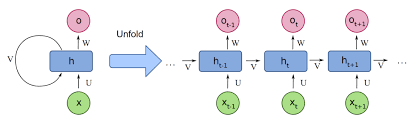
RNN: (1985)

Recurrent Neural Networks (RNNs) are a simple way of processing sequential data (in our case words and natural language). We have a hidden neural network (NN) that takes an input of the previous hidden state and new input, and spit out a new embedding. From that can make decent guesses at the next token in a sequence. A huge issue with these networks is that they have to be trained serially and that there’s an exploding or vanishing gradient. This is all matrix multiplication, so when your range of numbers lie below 1 it’ll tend to go towards zero, or if they’re greater than 1 they explode to infinity. So in essence this method doesn’t take in the context of surrounding words very well, can’t train well due to long sequences and the matrix multiplication causes vanishing and exploding gradients.

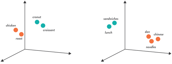
Word Embeddings: (2013)

A very interesting concept when I first learned about it, is that we can represent language with numbers. This first method we discuss in word embeddings doesn’t take into account much context, but is nonetheless an important first step in having a model understand language. We create nth dimensional vector representation of words through constructing a NN. This NN will try to predict the next word in a sequence through slowly changing the weights within its hidden layers. We are encoding context in every prediction within the hidden layer activations that serve to form the basis for word representation in a mathematical sense. The following demonstrates a simple 3 dimensional case where various words with similarities are closer than other non-related words.

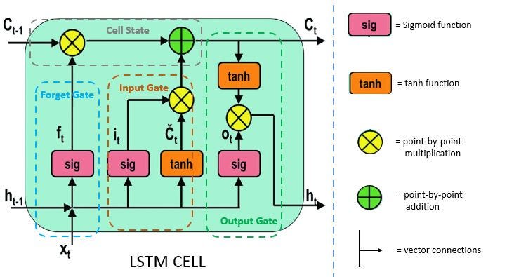
LSTM: (1997)

LSTM (Long Short-Term Memory) is sequential like RNNs, however they avoid exploding and vanishing gradients through having long-term memory and short-term memory channels labeled c_t and h_t. The sigmoid function in this case can be thought of capturing the “importance” of a particular activation as it squeezes numbers between 0 and 1, while the tanh function records whether something should be remembered or forgotten as it squeezes numbers between -1 and 1. These two functions are used a lot, and remembering them this way helps conceptualize the LSTM much easier. The forget gate tells us how important something is to forget. The input gate gives us how important something is to remember, and if that memory is a positive or negative value. Lastly the output gate determines our next short-term memory, or what lessons we take from our long-term memory in conjunction with the importance of our last short-term memory. LSTMs are great for attacking this vanishing/exploding gradient problem, they can remember key information for long periods of time and they generalize very well. Due to all the extra calculations though they train and execute slower and require more memory to adjust to the correct internal weights. There’s another architecture called a GRU that is a smaller, faster LSTM, however they aren’t as efficient and only serve as a detour to go into detail on.

Transformer: (2017)

For this one I’m going to take a little longer, as this is arguably one of the most important innovations of all time.

Firstly, this transformer design is used to translate language.

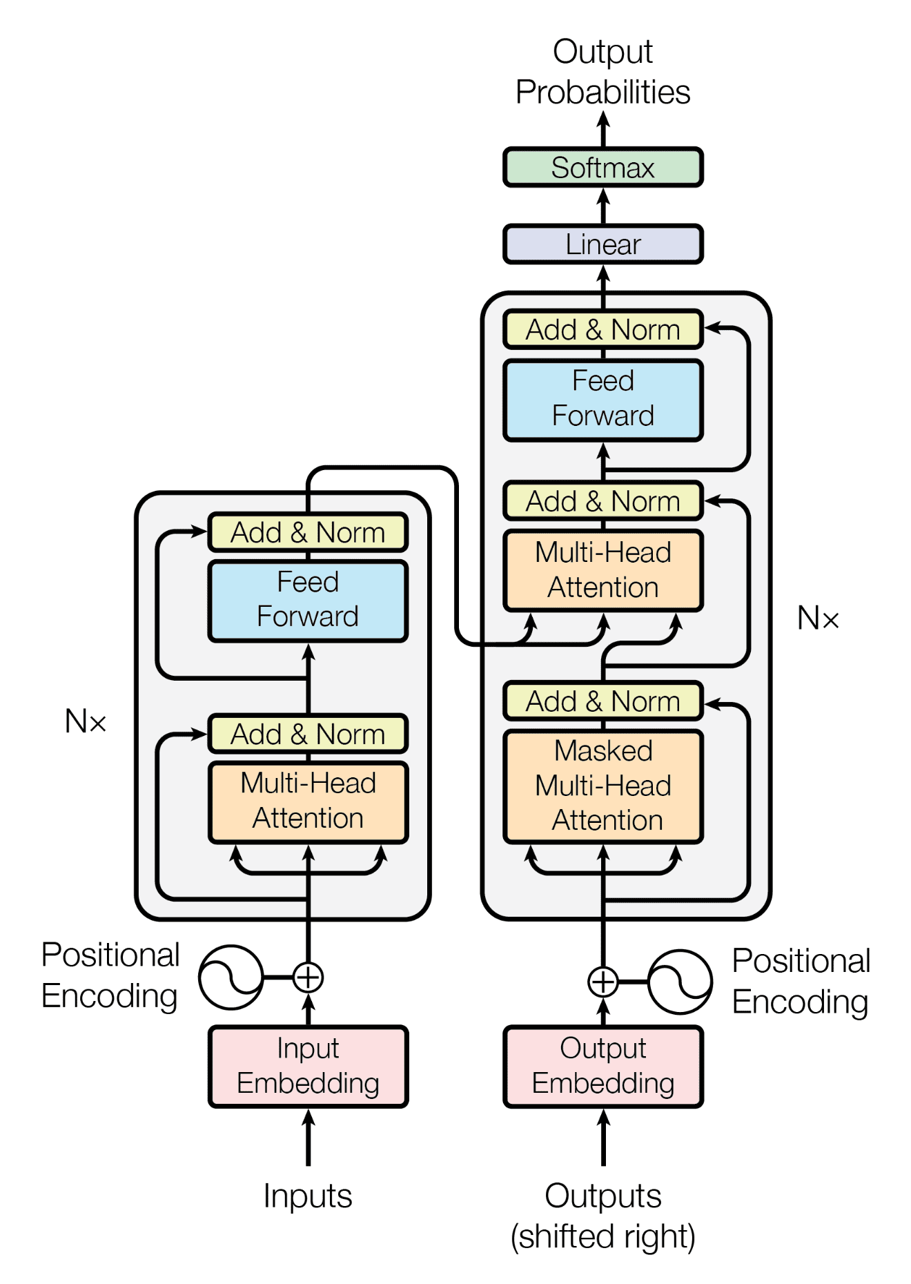
All the words in a sentence are passed through an embedding table that transforms a word into an nth dimensional vector.

The positional encoding is an alternating sinusoidal element-wise addition that is learned by the model such that it can distinguish the position of a word. We’re basically adding a super small value to our embedding such that the context of the word doesn’t change, but does enough to pick up on the positional context in relation to other words. Since we’ll be comparing words together (multiplying them), having unique interactions between the relative embeddings of words is why this technique works. We can concatenate positional encodings as well, but this increases the cost of compute. Another idea is to not include positional encodings at all, which for much larger models seems to be shown to be effective.

The next gray box is trying to encode a representation of the learned sequence. It has a multi-headed attention section and a fully connected feed forward network where both have residuals being concatenated forward to the next section so as to not lose any embedded information.

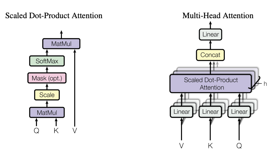
Attention is split into three variables: Queries, Keys and Values. We want to understand the word embedding Q. We take the dot product of each word embedding K by Q. This value determines the importance, and gives us a weight W. Each word embedding V is multiplied by their respective weight W and added together to get a final, contextualized word embedding. But what is being trained here? Well, before we take each Q,K and V, we multiply them by a Query and Key Matrix and Value Matrix. Each matrix is a weight to be optimized for such that our attention block can now learn!

Now, instead of using one scaled dot-product attention block we’ll instead use a series of separate blocks that are concatenated and fed through a dense layer to have the output of the word embeddings be the same size as the input! Each head of the network is a unique queried word being evaluated with every other word.

Because the size of the input is the same as the output and because the output is a vector of embedded contextualized words, we find that we can repeat this process Nx times. Nx is a hyperparameter that then can be used to iteratively improve results. The reason we are taking in the original signal and adding it to the value produced is because of resnet, and how in deeper networks we oftentimes lose signal in deeper layers. This method prevents the decay of loss gradients making the network more efficient to train.

As for the decoder block, we slowly feed in each new word one at a time, going “The” to “The cat” to “The cat went” etc. Each loop the network is essentially guessing what the next word is going to be given the context of the completed initial language and the previous words of the output string. This is how our network learns, it gets feedback on whether the correct word was predicted, and as you can expect, this takes a long time to train. The output’s encoding process looks similar to the encoding, except there’s a second multi-head attention block that takes in the input final word embedding and the output word embedding to add full context to both languages and do its best at predicting the next word.

BERT: (2018)

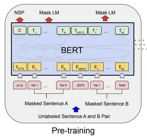
BERT’s pretraining phase looks to establish language and context. First, it makes use of a Masked Language Model (MLM). Adjectives can start before or after nouns depending on the language. One language puts adjectives before a noun and other languages put adjectives after. This means that we’ll miss crucial context if in our transformer model we start from left to right. Instead in BERT (Bidirectional Encoder Representations from Transformers) we randomly mask various words and have the model figure out given a bidirectional context of words. The second part in pretraining is to have BERT understand which sentences follow the next; a task called Next Sentence Prediction (NSP) that gives a yes or no given the word embeddings of both sentences. MLM and NSP are trained simultaneously as shown in the diagram above.

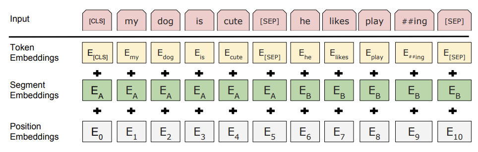
For the input embeddings we make use of a new way of describing words. We have our initial token embeddings and positional embeddings, but now we have segment embeddings which describe the beginning and end of segments.

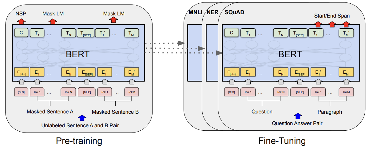
Next we start the fine tuning phase where we use the Q & A task to match questions with answers. A question is passed in as well as a paragraph containing the answer, and the output is made to be the start and end words of the answer in the paragraph.

GPT-1: (2018)

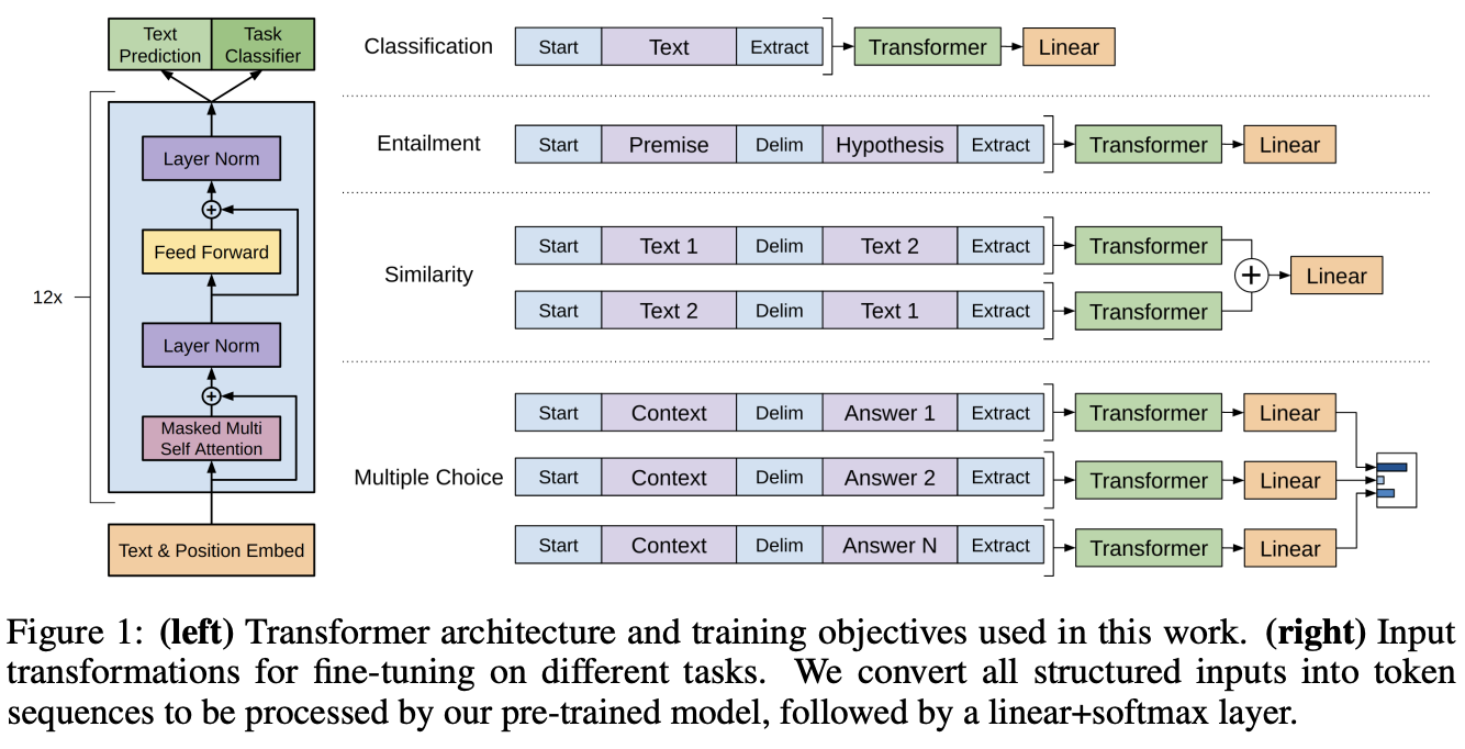
GPT-1 is broken first into an unsupervised pre-training task in which the algorithm is simply trying to predict the next token given a window of previous tokens. The next supervised fine-tuning task will feed in input tokens, look at the final transformer block’s activations, and use it to predict a new label y. These tasks are shown below to be classification, entailment, similarity and multiple choice.

BART: (2019)

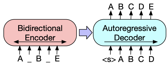
Similar to BERT, BART basically just adds more noise to inputs. Instead of token masking, we also switch around existing tokens, delete some others, and in general mess up the text as much as possible. Then all that BART does is do an initial bidirectional encoding just like BERT, and then use GPT’s autoregressive decoder to order and predict the next token.

GPT-2: (2019)

The previous GPT-1 model succeeded, but wasn’t very flexible and required supervised training. GPT-2 goes full unsupervised and expands the data trained on to achieve better performance. Feeding in unsupervised data by itself does not help, as a lot of large datasets like Common Crawl hold little intelligible data. Instead GPT-2 uses a subset of documents with a focus on quality.

A real-world model shouldn’t be limited by only using words, but should be able to make up words, use unicode bytes and do much more and have a level of flexibility. Current models using this more flexible design don’t perform as well as models that filter for words, but a middle ground was used in Byte Pair Encoding (BPE). Instead of mapping unicode with 130,000 base vocabulary, only mapping the bytes that comprise unicode results in a 32k to 64k vocabulary. This vocabulary breaks words down to prefixes, suffixes and sub-word instances. This allows for a better understanding of words and their relation to others.

Other than that, the dataset is larger and the transformer model is slightly altered to allow for more depth and scale.

GPT-3/4: (2020/2023)

GPT-3/4 basically uses the same architecture as GPT-2 but just feeds in more high quality data into a bigger model.

Final Thoughts

The field still has a long way to go, and I’ll want to make a part 2 at some point detailing further developments in the field, especially with relations to medicine. Thank you for reading! I hope this has been helpful in understanding such crazy technology. 🙂