The Biomedical Signal Processing Deep Dive

In my research and understanding of multimodal models in health, I came across a modality that I dreaded; unidimensional data. How do you deal with such a modality? What’s tricky is that unlike other modalities it isn’t discussed as much and oftentimes feels underdeveloped in the literature. With no formal training in how to deal with this topic, I went back and read the first seven chapters of “Biomedical Signal and Image Processing by Kayvan Najarian and Rover Splinter”. These chapters that I’ll cover the first five of momentarily discuss the basics required to proceed with research in the domain of biomedical signal processing.

After the book material I went to cover an MIT course in case I missed any general information and then looked at current literature. And while I originally only cared about 1D data, those techniques easily expanded to 2D data as well.

Book Material

Chapter 1: Signals and Processing

The most we really get from here is an introduction. Stuff like how a signal is a 1-D ordered sequence of numbers. Nothing too tricky. The authors differentiate between analog signals, discrete signals, and digital signals, as well as a general overview of processing and extracting features for analysis. (We’ll touch more on this later). This book goes into image feature extraction as well, which isn’t as useful given modern-day technological advancements in CNNs, but nonetheless are brought up. They will serve a purpose but again, we’ll touch more on this later.

Chapter 2: Fourier Transform

Immediately starting off with the heavy hitters we have fourier transforms (FTs). FTs are essentially the decomposition of signals into composite frequencies. Every wave complex can be made up of a group of sinusoidal waves oscillating at different frequencies, and FTs break down a wave into these smaller wave coefficients. The 3B1B video on FTs is one of the best, and starts off by discussing that of the “Almost Fourier Transform”, where by recording the center of mass of the signal spun around a circle gives us interesting properties. This seems incredibly unintuitive on why we’d make this step, and I get that, but it’ll work out nicely. What this does for us however is it means the center of mass is only really away from the middle of the circle when the frequency of the sign wave is the same, in which it forms a circle.

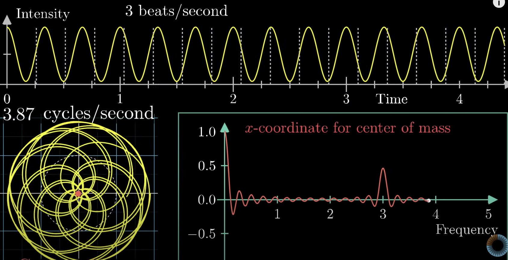
The x-coordinate for center of mass can be added and subtracted to get good approximates of the original signal. The original signal is spun around this circle and then can be decomposed around unique frequencies that build up the original signal. Before we get to the actual FT let’s build up the math. The actual way to rotate about a circle clockwise is to use imaginary numbers. The expression below demonstrates this ability to circle around the axis where t is time.

\[e^{-2\pi it}\]

We can then multiply by the frequency f that controls the speed of how fast we go around the circle. The intensity as a function of g(t) multiplied to the equation allows us to do our better FT. The center of mass then corresponds to the following integral:

\[\frac{1}{t_{2}-t_{1}} \int_{t_{1}}^{t_{2}} g(t)e^{-2\pi ift}dt\]

But we don’t actually care about the center of mass, we can get rid of the 1 over t2-t1 and just scale up our center of mass vector by multiplying our value by the number of seconds.

\[\int_{t_{1}}^{t_{2}} g(t)e^{-2\pi ift}dt\]

We have to take discrete measurements and try to form a continuous signal. To have confidence we’re not missing anything we find the fastest frequency in our signal and make sure we’re recording twice as fast as the fastest signal. This is referred to as the Nyquist rate. Because we can only measure in discrete measurements, we have the discrete fourier transform (DFT) as the following equation:

\[X_{k} = \sum_{n=0}^{N-1} x_{n}e^{-2\pi i * kn * \frac{1}{N}}, n=0,...,N-1\]

For N complex numbers x_{n} into another sequence of complex numbers X_N.

Inverse transformers exist for both reverting the continuous and discrete FTs to their original state. No information is lost in this process. FT can have hard cutoffs for low-pass filters to eliminate noise, but also softer caps such as the Butterworth filter that gradually eliminates noise to eliminate noise while having a more uniform sensitivity for desired frequencies.

Chapter 3: Image Filtering, Enhancement and Restoration

So now we’re getting into images for a moment. Some of these techniques are still very useful when in conjunction with more modern methods. At the end, we’ll see how a hybrid of traditional methods combined with newer methods always seem to perform the best, though they require expertise and finesse to pull off.

Point processing is any simple transform in which it takes place on an independent pixel by pixel basis. Construct enhancement involves spreading the greyscale more evenly throughout the image to decrease the contrast. Histogram equalization has all gray values equally related by filtering larger instances of gray into neighboring buckets.

Median filtering can be used to help eliminate drastic sources of noise in images.

That’s really it for this chapter. It’s quite simple, as imaging techniques are simple and easy to understand in comparison to unidimensional biomedical signals.

Chapter 4: Edge Detection and Segmentation of Images

Developing a kernel that’s sensitive to specific shapes is discussed in this chapter as an effective way to determine key information about the boundaries of images. These are common in CNNs so I won’t go into much detail about them here, but they’re great for edge detection.

The rest of the chapter is more outdated tech like region segmentation that is now done much better with modern ML segmentation algorithms.

Chapter 5: Wavelet Transforms

The issue with FT is that they don’t take into consideration the timing or order of data. We can have a frequency of a wave come up in the middle of a longer signal, and while we can see its frequency representation as a whole on our fourier transformation, we don’t know exactly when specific signals occur. The best strategy is then to use a wavelet to detect our specific wave we wish to see. A wavelet is a rapidly decaying wave like oscillation that has zero mean. To choose the right wavelet will depend on the application it is being used for. Scaling a wavelet stretches or shrinks it horizontally. It can be shifted as well along the time axis. A continuous wavelet transform is defined as the following:

\[W_{\psi ,X}(a,b) = \frac{1}{\sqrt{|a|}} \int_{-\inf}^{+\inf}x(t)\psi^{*}(\frac{t-b}{a})dt, a\neq 0\]

where a is the scaling parameter and b is the shifting parameter. Ψ(t) is the mother wavelet multiplied by our signal x(t). This integral can then give us the integral over the matching parts of the wavelet and signal, meaning the resulting value will be a value representing the likeness. Note that this is also normalized by the constant a.

This would then be the discrete wavelet transform:

\[W_{\psi, X}(a,b) = \frac{1}{\sqrt{|a|}} \sum_{i=0}^{N}x(t_{i})\psi^{*}(\frac{t_{i}-b}{a}), a\neq 0\]

In wavelet decomposition, the input signal is convolved by two wavelets, a low-pass (approximation) wavelet and a high-pass (detail) wavelet. The low pass portions are iteratively filtered again and again by a low and high pass filtering process.

A signal’s approximation is the in between values of two previous points. This results in half the number of points. The detail is then the difference between the two previous points. This way we have a transform of two types that work as a low pass and high pass filtering system.

These signals are iteratively filtered to gather coefficients (the approximation and detail numbers that are calculated) in order to decompose a signal into more usable sections.

The Daubechies (dbX) wavelets are a collection of waves starting from 1 and going to 20. They start off rough and long and slowly over time increase in frequency and smoothness. There are other mother wavelets, however a rule of thumb is the one we choose should match the complexity of the signal and the shape of the signal we wish to catch.

Discrete wavelet transforms are used for denoising and compression of signals and images. The process for applying wavelets first starts with us having a low pass and high pass filter on the input signal. Then we apply the same two filters on the smaller low pass filter (each time this is called a bank). Wavelets are analyzed on the high pass filters for each bank.

MIT Course Additional Information

Whenever I want to learn material, even for a class I have I’ll refer to the best places I can find information. Generally Stanford, MIT and Berkeley put out content where the professor is 100% confident in what they’re putting out. This may not be the case in other institutions where a student can oftentimes gamble with the teaching ability and/or knowledge of the professor. Here are a few notes I took from the MIT course that the book did not cover.

The only material that I didn’t see covered in the book that was in the MIT course was that of some digital filtering techniques.

A finite impulse response (FIR) is the reaction to a sudden and instant impulse (change). This oftentimes is measuring noise, so FIR filters remove said impulses. Filtering that goes on longer can be referred to as IIR filters (infinite impulse response filters). This is often due to feedback that decays over time. The use cases for both filters here are more nuanced than what I’m letting on, but if processing raw signal data is proving difficult due to sudden jolts or movements causing unwanted noise, these are a good option in one’s toolbox to delve further into.

Research

Now we’re getting into the practical applications of various biomedical signals in health! Let’s begin with modern research!

(2015)A new contrast based multimodal medical image fusion framework

This paper uses the non-subsampled contourlet transform (NSCT). The NSCT is a form of wavelet decomposition that takes into consideration 2D multi-scale and multi-direction information. The method decomposes the source medical images into low and high frequency bands in the NSCT domain. Differing fusion rules are then applied to the varied frequency bands of the transformed images.

Low frequency bands are fused by considering phase congruency. Phase congruency compares the weighted alignment of fourier components of a signal with the sum of the fourier components. This captures the feature significance in images and is particularly good at edge detection. High frequency fuses on directive contrast. Directive contrast “collects all the informative textures from the source.” As a result we get a desirable transform on medical images that preserve image details and improve image visual effects for the purpose of diagnosis.

(2018)Deep Learning on 1-D Biosignals: a Taxonomy-based Survey

Surveys are great sources for understanding where a field is in terms of progress and where a researcher ought to focus their attention. The paper introduces the field of 1 dimensional biosignals describing biosignals as generally non-linear, non-stationary, dynamic and complex in nature. This means that creating hand-crafted features to test on is not reliable.

The paper talks about how a common practice is that of using pretrained NNs, as small medical datasets aren’t enough to effectively train many NNs.

Issues often not considered in 1-D biosignals is that of how training and collecting data with specific medical devices will give different results to that of other similar devices. Either there’s an issue with sampling rates, or preprocessed steps that modify the data in undesirable ways. Another issue discussed is that clinical significance can only really be gathered from multimodal analysis. Luckily I’ll be doing a major post on that next!

Most techniques brought up seem to fail in capturing meaningful data from biosignals due to their inability to handle the complexity of the data being dynamic and multivariate.

Deep learning is the current candidate for deep learning data as it’s able to handle the multimodal data required and is currently mostly limited by data acquisition issues, hence pretraining being so abundant.

Lastly, Multi-lead CNNs and LSTM models are used for clustering tasks while autoencoders are used for signal enhancement and reconstruction tasks in general at this point. Note that this survey is in 2018, and developments do move fast, though it’s good to note trends and how specific algorithms benefit in various ways.

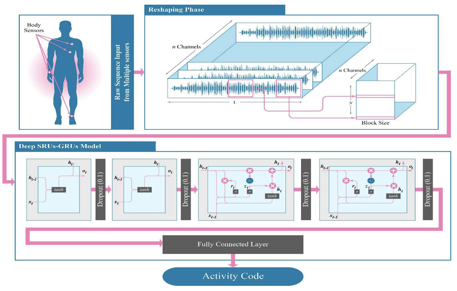
(2019)A Hybrid DL Model for Human Activity Recognition Using Multimodal Body Sensing Data

Given multimodal data for biosensors, this paper wants to predict what a person is doing (e.g standing still, bending knees, running, etc).

SRUs, GRUs and LSTMs are proposed for handling the health data, though the authors drop the mention of LSTMs for an unknown reason. The SRUs just add both input and hidden state and do a tanh operation. That’s it in case this was an unfamiliar architecture to anyone. They function as a simpler GRU and are shown in a diagram below.

THe proposed solution “solves” this problem, achieving almost 100% accuracy. All it does is stack two SRUs followed by two GRUs together. The model takes in 23 inputs from the differing health channels collected.

It is suspect that the results are so good, as nothing in this field comes close to this level of consistent performance. Maybe the training and testing data got mixed up somehow? Otherwise, the algorithm chosen is quite interesting and could be used for future signal processing purposes. It doesn’t have much to do with our biomedical signal review, but this next paper leverages them wonderfully.

(2019)A comparative review: Medical image fusion using SWT and DWT

Image fusion is the process of combining multiple images, resulting in a single image. The authors perform Stationary Wavelet Transforms (SWTs) and Discrete Wavelet Transforms (DWTs) to determine which are better.

Well why don’t we just stack images on top of each other and forget this whole wavelet nonsense?

1. We may have different resolution images.
2. Edges may not be exactly preserved.
3. We may have noise and artifacts.
4. There may exist incorrect exposures of each image.

Discrete wavelet transforms are used as a filter, breaking down the image into fundamental coefficients that represent signals of the image. This combats multiresolution issues, noise, and can be fused well before inverting the coefficients to an image again. They’re also great with dealing with edges.

Because discrete wavelet transforms are discrete, and therefore shifted over an image they’re known to have “translation invariance”. They work the same irrespective of where they are. But this means it may be poor if we need context sensitivity, or take into consideration spatial relationships or localization. This can lead to overgeneralization very easily.

We use stationary wavelet transforms to fix this, and on their own they’re preferable to DWTs. DWT and SWT are combined and we use the inverse SWT to get our final image that fuses both wavelet transforms for ideal results!

(2019)Multi-method Fusion of Cross-Subject Emotion Recognition Based on High-Dimensional EEG Features

This paper focuses on determining the emotional state of a subject given feature extraction from EEGs. Before we get into that we have to discuss more reviews that weren’t discussed earlier.

1. Hjorth Activity: The power spectrum.

\[Activity = var(y(t))\]

1. Hjorth Mobility: The mean frequency, proportion of standard deviation of the power spectrum.

\[Mobility = \sqrt{\frac{var(\frac{dy(t)}{dt}}{var(y(t)}}\]

1. Hjorth Complexity: The change in frequency.

\[Complexity = \frac{Mobility(\frac{dy(t)}{dt})}{Mobility(y(t))}\]

1. Simple standard deviation.

Before we can talk about sample entropy and wavelet entropy we need to understand entropy. Entropy is our surprise. When the event of an outcome is low we want a lot of surprise, while the closer it is to 1 we want 0. The inverse log suits this perfectly. The entropy of a process can then be the average of the surprise for each outcome; entropy is the expected value of the surprise.

If we have a loaded coin with the following table:

	Heads	Tails
Probability	0.9	0.1
Surprise: log(1/p(x)	0.15	3.32

The expected surprise (or entropy) is then:

\[=(0.9\cdot0.15)+(0.1\cdot3.32) = 0.47\] \[\sum xP(X=x)\]

where x is the surprise, let’s replace x with the probability of the event and simplify.

\[Entropy = -\sum p(x)log(p(x))\]

If we had a fair coin the entropy would be 1, while the smaller to 0 we get the more entropy exists.

1. Sample Entropy: Calculates the unpredictability of waves by comparing wave signals to see how similar they are. It looks at two sets of simultaneous data points and compares their similarity in comparison the a slightly wider window.

\[SampleEn = -ln\frac{A}{B}\]

A and B are the summations of logical comparisons between values in a sliding window. This means that similar values will be added up together. If there’s a lot of similarities we’ll get 0, but if there’s no consistency in windows we’ll get a higher value. The window size and what contitutes the same value within a specific threshold will change the sample entropy recorded.

Another way to picture this is that a flat line will result in the two windows recording the same number of similar points, resulting in 1 (the negative log of 1 is 0). In a less predictable signal we’ll get a good approximation into the entropy as the larger window is drastically better than the slightly smaller one, ultimately causing more entropy to occur.

1. Wavelet Entropy: Does wavelet decomposition and then computes an entropy measure on the coefficients.

Next are four PSD frequency domain features:

1. The power spectral density (PSD) is the fourier transform of the autocorrelation function of the wave. So if our signal is noise, correlation is zero, and our fourier transform is a flat line. The power spectral density is then a constant. However a square wave form produces an autocorrelation function of an isosceles triangle around the origin. The corresponding PSD is then a sinc squared function shape. Our PSD was then used on four preprocessed rhythms alpha, beta, gamma and theta.

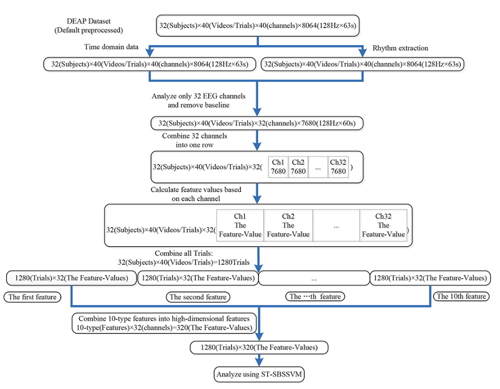
In this diagram the final ST-SBSSVM method is a significance test (ST), sequential backward selection (SBS) and a support vector machine (SVM). SBS is a significance test in which variables are eliminated until only the variables that are statistically significant relative to the SVM are left.

(2020)On Instabilities of deep learning in image reconstruction and the potential costs of AI

This paper talks about how current technology for image reconstruction is still best done with FTs as deep learning can often remove the tumors or other abnormalities we want to observe. This makes complete sense as deep learning is trained to reconstruct the near average of what it sees and remove artifacts that may be important.

ML may be thrown off by artifacts and this can cause severe errors in reconstruction. Like how a well placed black box on an image of a cat can result in it being recognized as a fire truck. There can even be a case where the more images fed in can cause the quality of restorations to deteriorate as deep learning fails to take into account abnormalities and causes the algorithm to become more unstable.

(2021)A survey on deep learning in medical image reconstruction

This study goes off of the previous study quite well and adds some additional context to the progression of medical image reconstruction.

There have been three phases of reconstruction technology.

1. Fourier Transforms are efficient but require proper sampling.
2. Iterative methods like wavelets and total variation take into consideration the statistical and physical properties of the imaging device, but there are discrepancies between the model and physical factors like the inhomogeneous magnetic fields that can distort results.
3. With ML, images can be reconstructed from poor quality data, but they’re not computationally efficient and require a large set of balanced training data. This balanced training data is hard for medical domains and because so can be unstable as shown in the previous study.

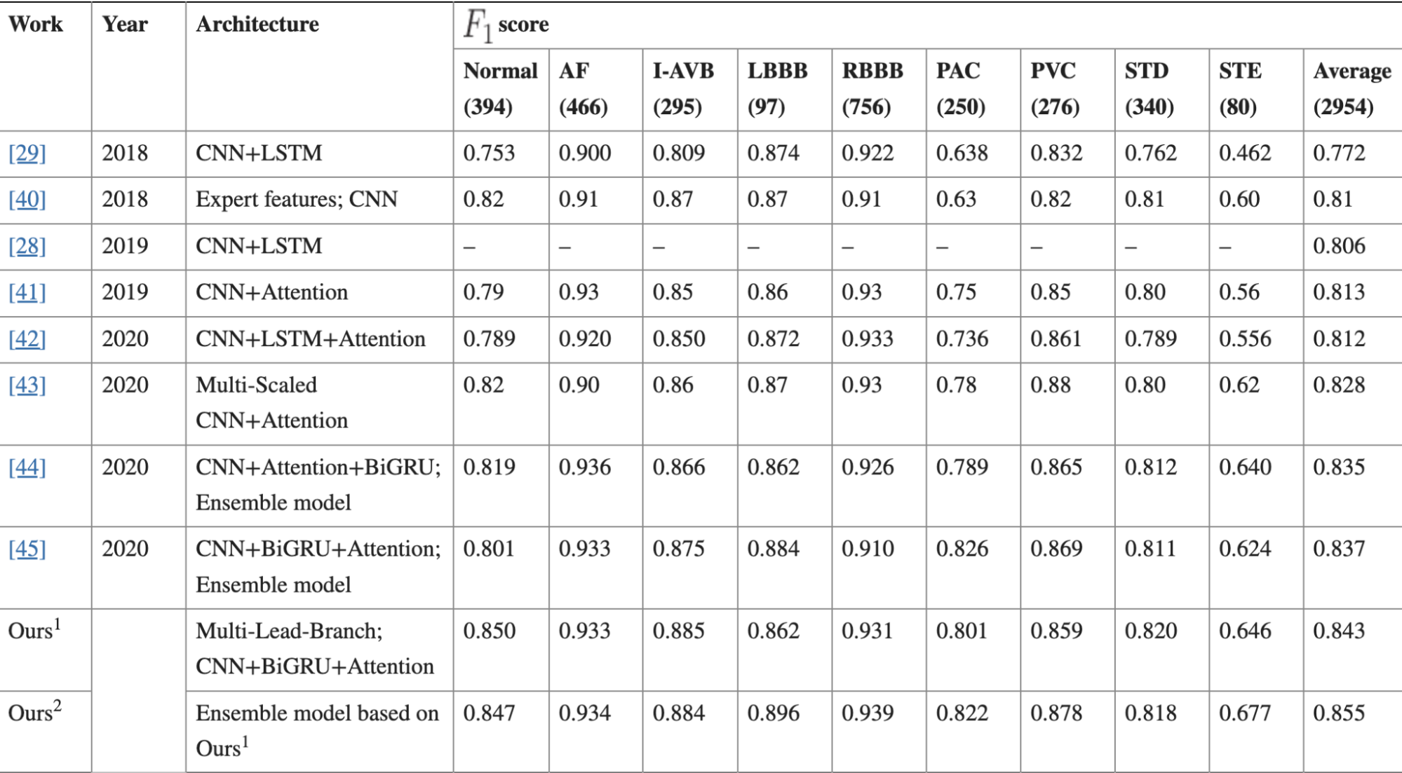
(2021)MLBF-Net: A Multi-Lead-Branch Fusion Network for Multi-Class Arrhythmia Classification Using 12-Lead ECG

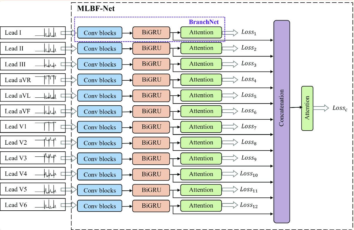
We have 12 inputs from our ECG data. All are fed into individual convolution blocks; 5 blocks with a total of 15 convolutional layers all together. Next we feed our data into a bidirectional GRU (over the LSTM for less computational complexity). Our encoded BiGRU is fed into a “one-layer multilayer perceptron” and a softmax layer. The one-layer multilayer perceptron is a little bit of an oxymoron but I think it’s just a single layer as the authors describe the layer as such:

\[u_{jt} = tanh(W_{w}f_{BiGRU_{jt}}+b_{w})\]

All the values are concatenated and fed ito one last attention network.

(2022)A review on multimodal medical image fusion: Compendious analysis of medical modalities, multimodal databases, fusion techniques and quality metrics

This is the last paper and is mostly for future work for if I need to pursue the topic of 2D data in the future. While this wasn’t originally related to unidimensional biomedical data, a lot of the same techniques ultimately were used for the same when applied to 2D or even 3D images. I also found a lack of clarity in the use of the term fusion. Multimodal fusion can refer to different types of images rather than entirely different domains being fused as well. A lot of this research was conducted as an extension of my original focus on multimodal data techniques.

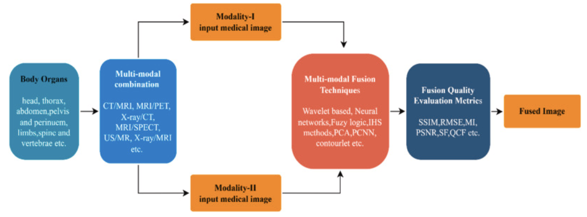
Multimodal fusion in this case is in reference to only that of early fusion techniques. And these techniques are shown to be numerous and complex as shown in previous descriptions of techniques utilized.

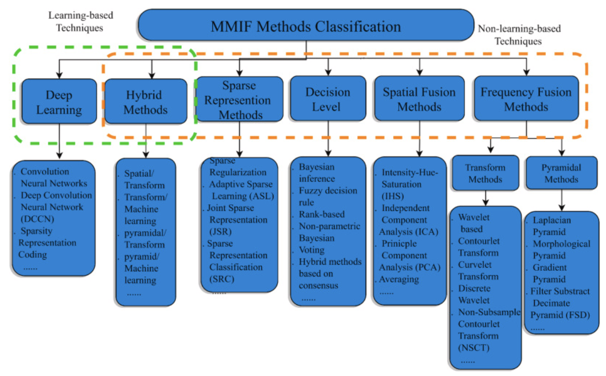
The paper summarizes the following about this long list of techniques used in the field:

• Frequency Fusion Methods:
  • Good quality option that can be used at multiple levels to great effect.
  • There may be less spatial resolution in the process.
• Spatial Fusion Methods:
  • Easy to perform.
  • Causes spectral degradations and isn't sharp.
• Decision Level Methods:
  • Improves feature level fusion by reducing unclear information.
  • Is incredibly hard to utilize and is time-consuming and complicated.
• Sparse Representation Methods:
  • Retains visual information better and improves the contrast of the image compared to other techniques.
  • Preserves information related to structure.
  • Can often produce visual artifact results in the reconstructed image.
• Hybrid Methods:
  • Minimizes artifacts, improves clarity, contrast, texture, brightness and edge information in fused images.
  • Requires detailed knowledge of each technique and how exactly to apply making it incredibly time consuming and cannot be used for large input datasets. (It isn't exactly stated why large input datasets are a challenge, possibly due to complexity issues?).
• Deep Learning:
  • Incredibly easy to optimize for and achieves excellent results.
  • Requires a lot of data and specialized care to get good performance.

Aaaaand that’s it! That is the up-to-date deep dive of biomedical signal processing! This was a smaller part of my bigger topic on multimodal models in healthcare, and I kept seeing tricky terms used surrounding this topic so I took the time to really delve into the meat and potatoes. Not all the papers I read were mentioned here, as this is already long enough, but this hopefully gives us a good feel for where the field is today and what techniques may be useful given certain modalities we wish to utilize in our analysis!

Thank you for reading, I truly have no clue why you did unless this is also a specialty you’re studying! :)