The Data Imputation Deep Dive

An interesting phenomenon in data is that of missing values. What’s even more interesting are the ways missing values mean different things. They can be missing completely at random (MCAR), but more likely there is a cause for why that data doesn’t exist. If we have other pieces of data that suggest why a value might be missing (missing at random: MAR), then not having a value is a value in itself that carries statistical significance. If the value is missing for a reason that only relies on the result and is outside of our control (missing not at random: MNAR), then we again have to take it into account in our statistical analysis.

For example, say we’re conducting a study on a hair growth serum.

MCAR would mean that a collection methodology might’ve broken, say the way we process data means every third person on hair growth serum gets their results deleted.

MAR would mean that there were people filling in surveys before the trial, and those who were displeased with the results stopped responding and dropped out of the trial.

MNAR would mean that there were people displeased with the results, as the hair serum didn’t work, however we have no corroborating evidence to suggest why they dropped out.

Also consider the combinations of these issues. We may have just one type of missing data, but we may have combinations of two, or all three present in our dataset.

Medical data is often sparse; we can have a lot of possible information presented, however very few is often supported for analysis. In many trials scientists can become lazy and simply drop out incomplete patients without a proper consideration into why data may be missing. Medical imputation is thereby the practice of understanding why we have missing data, and even the analysis of how best to alleviate the harms of missing data.

Listwise deletion is the simple process by which we delete any incomplete row. Pairwise deletion is the same as listwise deletion, except if the values we’re assessing are from X, Y and Z, and we are only conducting an analysis on X and Z, then we only remove values in which X and Z are missing rather than all three.

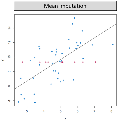
Mean imputation replaces missing values by the mean of their observed values. This distorts the distribution in several ways. A bimodal distribution is created that augments the data significantly and disturbs any statistical analysis we wish to conduct as most importantly, it drastically disturbs the relationship between variables.

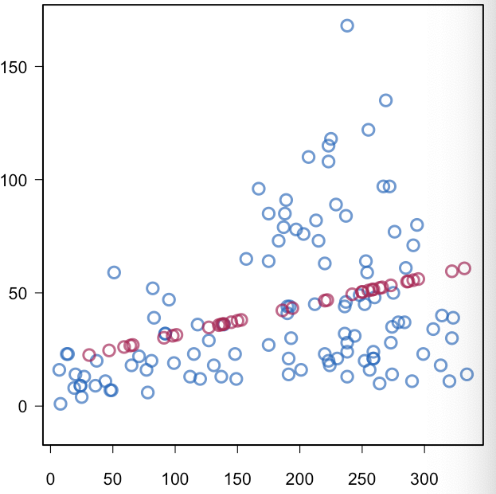
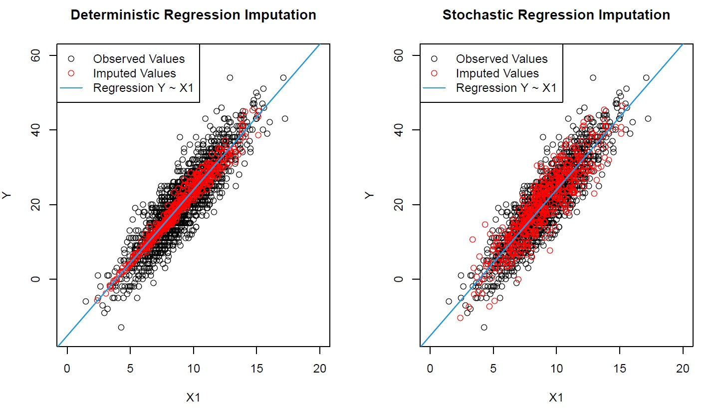
Regression imputation draws a linear regression line to match what the variable would be better, but there’s less variability in the original data. This is dangerous, as regressive lines may give an improper indication of whether two variables are truly correlated by making too many assumptions. This technique provides data that is “too good to be true”.

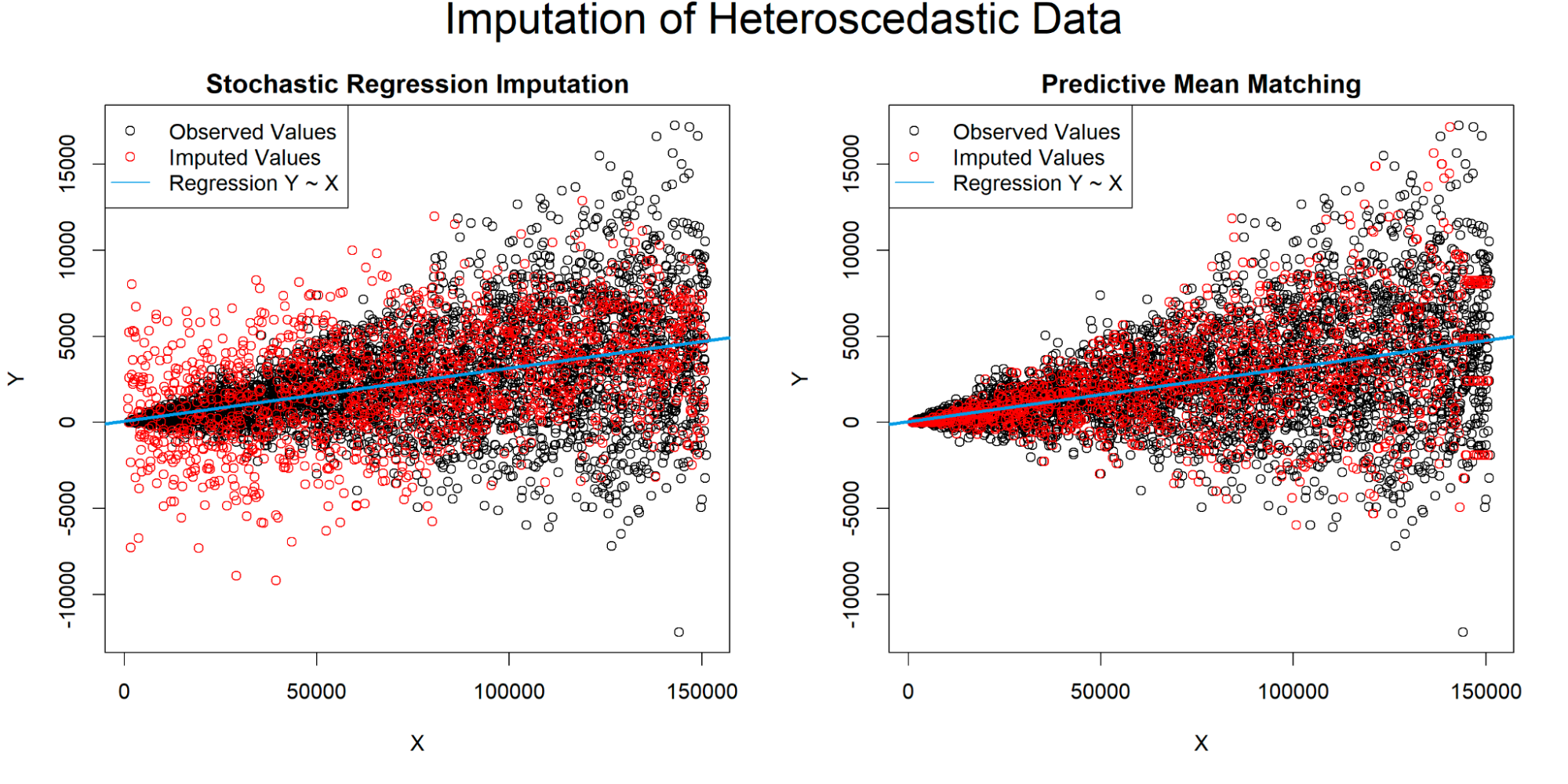
Stochastic regression imputation plays off of regression imputation, but instead adds noise to better represent an accurate standard deviation and variance of values. It works better and functions as a good baseline test, but still may overplay its hand in assigning correlations between uncorrelated variables.

LOCF (Last observation carried forward) can be good for time series data and can be found useful in some use-cases. However BOCF (baseline observation carried forward) is hardly ever used nowadays.

The indicator method tries to make “missingness” a feature, however it fails as a generic method to handle missing data and isn’t really used in current day practice.

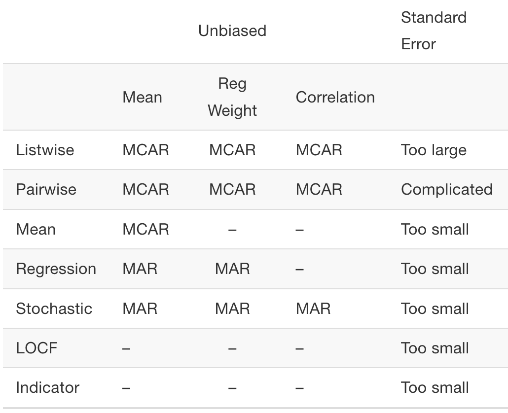
This table demonstrates the places where existing methods may be unbiased. Note that even when these imputation techniques are unbiased, they’re still underestimating or overestimating the standard error.

For traditional statistical analysis we get to the best technique: Multiple Imputation. Multiple imputation is best understood through its counterpart single imputation. Single imputation just assumes that the imputed value is treated as the true value. Then, in contrast, multiple imputation takes many differing imputations and finds the best values to treat as the true value.

All of our previous techniques beforehand were single imputation techniques that all misrepresented standard deviation, variance, standard error, and other statistical parameters. However with multiple imputation we can better select for a more accurate real value.

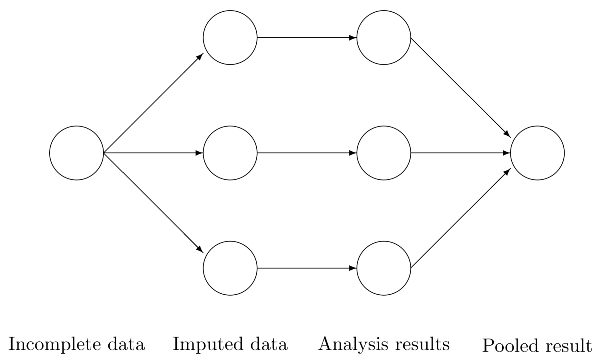
Multiple imputation has three steps:

1. Impute missing values with values randomly drawn from some distributions to generate m complete datasets.
2. Perform analysis on each m dataset.
3. Pool the m results and calculate the mean, variance and confidence interval of the variable.

This seems nebulous, and you’re right! Multiple imputation is implemented in many forms and most bootstrap another process called multiple imputation by chained equations (MICE).

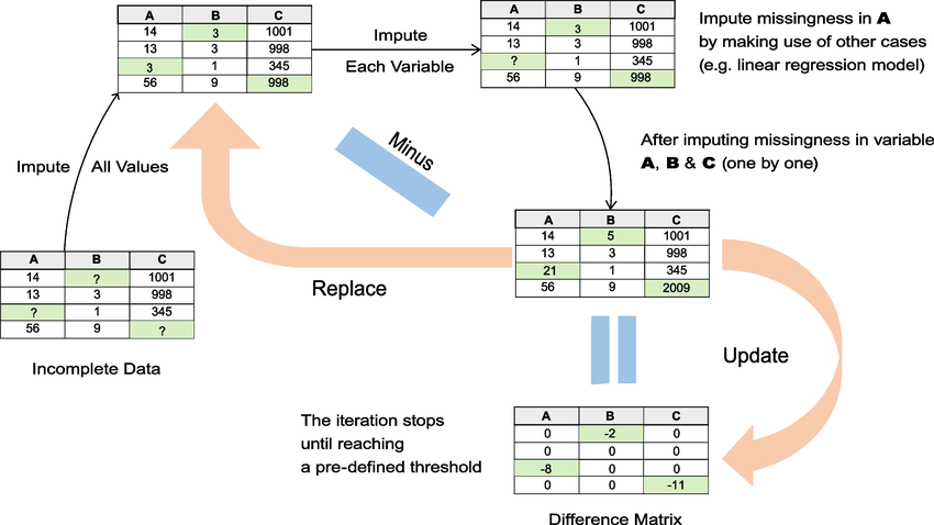
1. Impute missing values with values randomly drawn from some distributions to generate m complete datasets.
2. For each imputed dataset, impute missing values (that were replaced with guesses from out distribution) one variable at a time. Iteratively do this for all values in each dataset. We’re using a predictive model of some sort to guess the value that is missing.
3. Iterate this process of chaining predictions of missing values multiple times until an equilibrium is reached.
4. Pool the results using regression, hypothesis testing, etc. Use these pooled results to find the best values to fit into a single, final dataset.

This again doesn’t answer what exactly we’re using to make predictions on variables. We can use all of the previous single imputation techniques brought up, or other regression techniques such as random forests (MissForest), MICE with linear regression (MICE-LR), or MICE with denoising autoencoders (MIDAS). This is by no means a comprehensive list, just a list of the most commonly used implementations of MICE.

MICE can suffer performance-wise when the data is large or complex and has a high number of nonlinearities and high dimensionality. It is designed primarily for MAR, and works only decently on MNAR. Also, this technique is primarily used for static tabular data. This doesn’t get far in ways of time multimodal data and especially imaging data.

What other techniques are used? It may be important to know what techniques are out there that are utilized in data imputation, so here is a list with the most common baseline techniques used. Most of these baselines and future methods will come from this survey paper from 2023.

Traditional Imputation Methods:

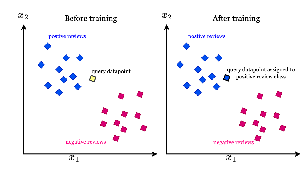
k-NN: Values are assigned on an n-th dimensional graph where a new piece of data that is incomplete is labeled by which points it’s closest to. This looks at the K Nearest Neighbors to find a consensus.

PMM: For quantitative values that aren’t normally distributed, predictive mean matching (PMM) is good. It essentially is just a different version of KNN where it looks at a small set of similar points and picks one at random.

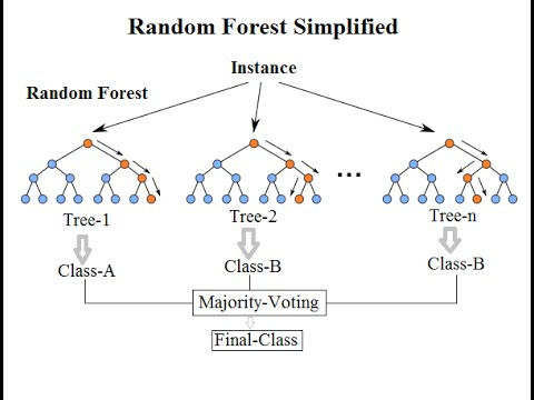
RF: A random forest is a classic bagging technique in which a decision tree is broken into a subset of smaller decision trees that vote on an imputation value.

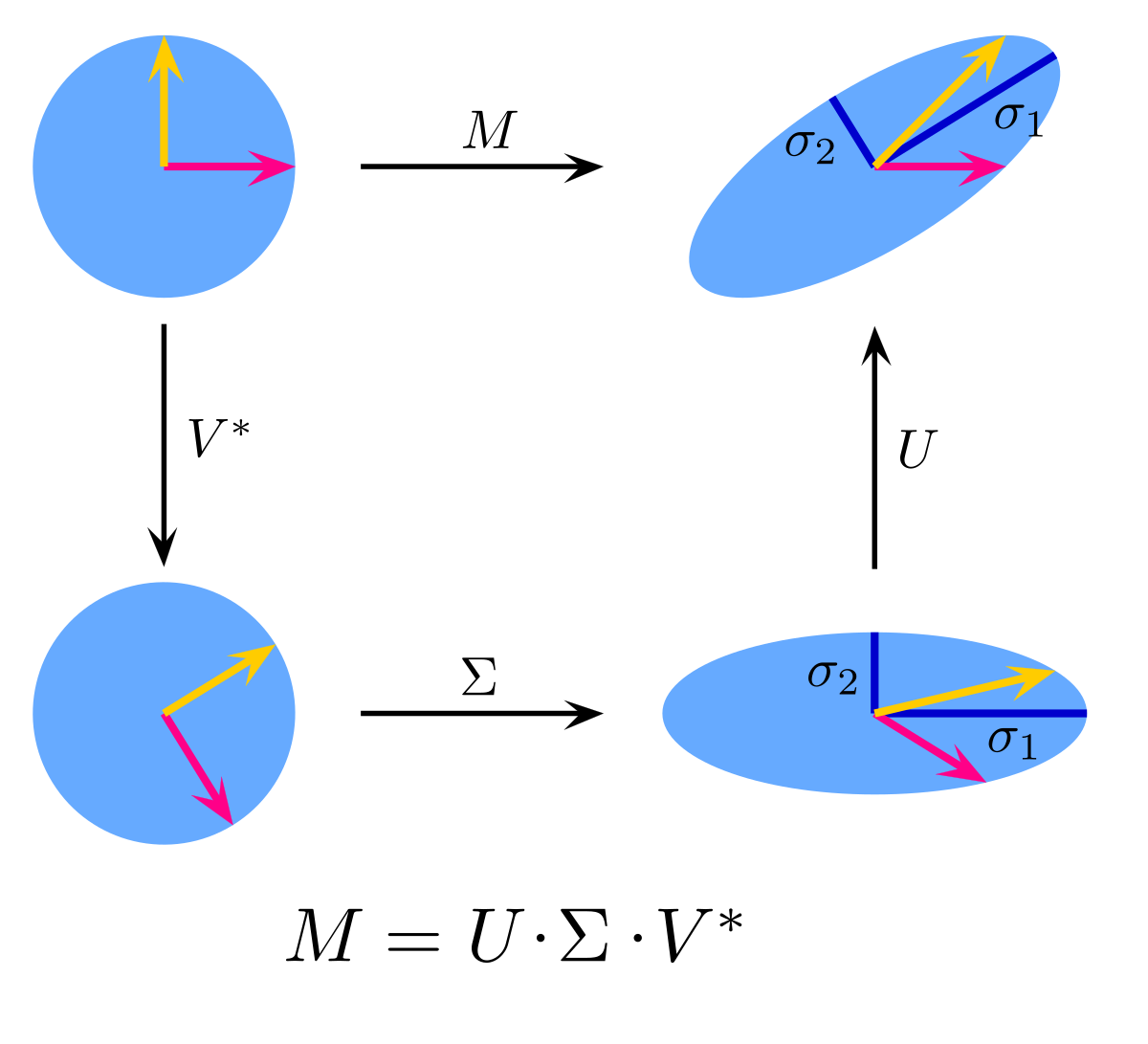
SVD: Singular value decomposition breaks down a matrix into three matrices. The first and third are rotation matrices and the middle one is a diagonal scaling matrix. The largest value in our diagonal matrix Σ is considered to have the most variance, or importance to the formation of the original matrix. This can be used to estimate missing values only after the missing values are initially filled in with some value.

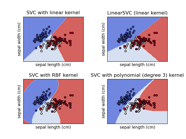
SVM: Support vector machines match a line, or a variation determined by a kernel to data points such that the value of incorrect placements is minimized.

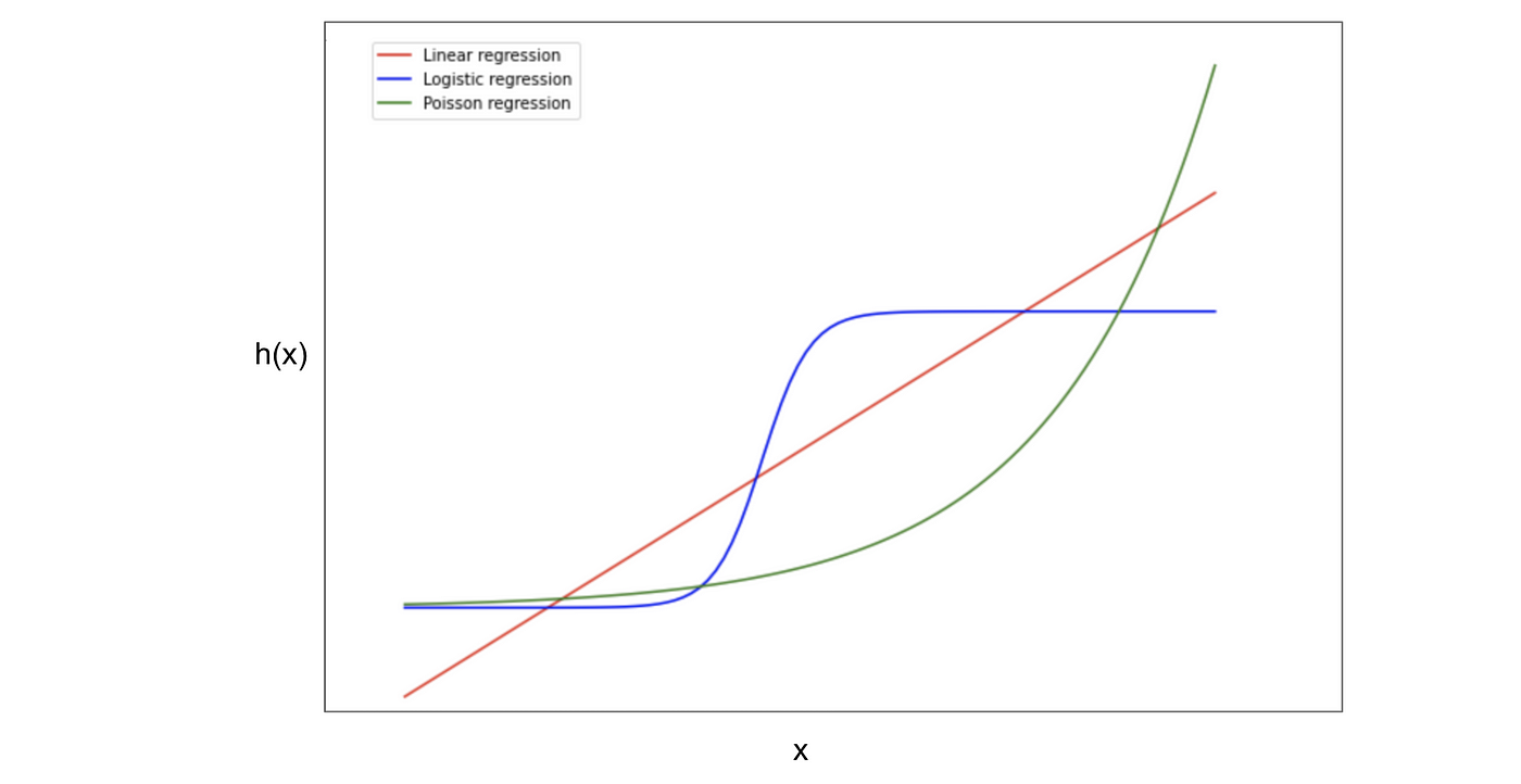
GLM: Generalized linear models start with a systematic component. This is our y=mx+b that describes how the input is related to the output. The link function is what will bend our systematic component; it bends the line. The final random component is the distribution we wish to use. This is basically the framing of a simple linear regression model into whatever form we wish to utilize it in.

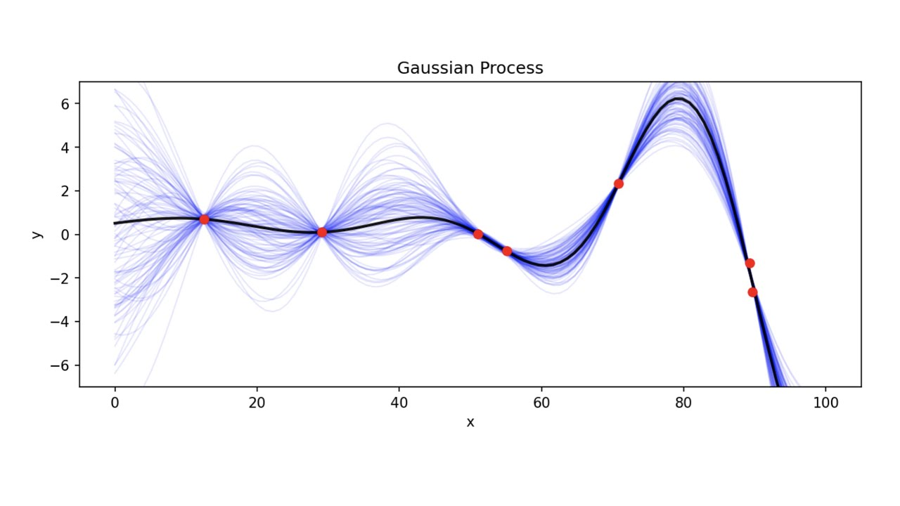
GP: Gaussian processes are a cool way of fitting a predictor. Say we have a linear regression task, we can develop variance and uncertainty about the points, but GP takes into consideration the uncertainty of the line itself. A kernel determines which type of functions look to fit to the data and takes tuning and knowledge to get right. For instance, we can add various kernels together to model very specific trends in data.

MCMC: Markov chain monte carlo can be broken first into two parts. A markov chain is a finite state model by which the chance of going to a new state is determined by an expressed probability.

A monte carlo simulation is a simulation by which we have a mathematical model as well as a number of random variables and then let multiple simulations run their course to see the range of possible outcomes.

Inverse transform sampling takes a distribution such as a uniform distribution and can turn it into an exponential distribution. Find the inverse of the desired distribution’s CDF (we get a function that we use as a transformation, in our case exponential to uniform). Plug in the uniform distribution into this function to get the new exponential distribution. In order to sample from this distribution we need an explicit formula for the CDF, which we may not have.

In accept reject sampling we have a target function f(x), but have a hard time sampling from it. We create an easier proposal distribution function g(x) and make sure the area it covers is always greater than the target function C*g(x). g(x) would be better as a normal distribution as to minimize the reject region of this graph.

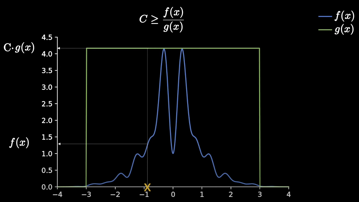
We choose a random point in our distribution, and take a uniform sample from 0 to C in which we can accept the sample or reject the sample, depending on if it is greater or lower than the blue line. Randomly sampling a bunch of times means that our acceptance density is the same as if we were to sample from f(x).

I had the idea here of combining gaussian mixed models and wavelet transforms, but unfortunately this idea was done. 🙁 Makes me feel good about my intuitions of math though. 🙂

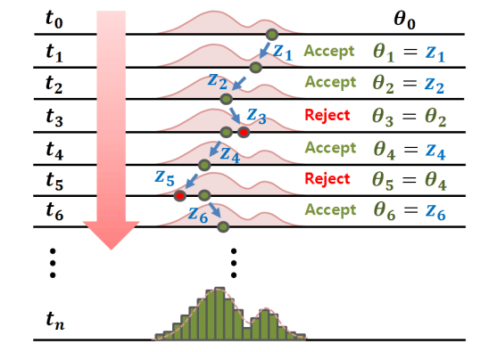
Lastly, in MCMC we improve upon where we sample. We design a markov chain to represent a discrete number of nodes and as we conduct accept reject sampling we adjust the probabilities of various transitions until we hit a stationary distribution, by which sampling from said distribution is the same as sampling from f(x). This is used in multiple imputation by combining sets of imputed datasets and finding a final distribution through MCMC estimation to draw from and impute.

Matrix Completion Imputation:

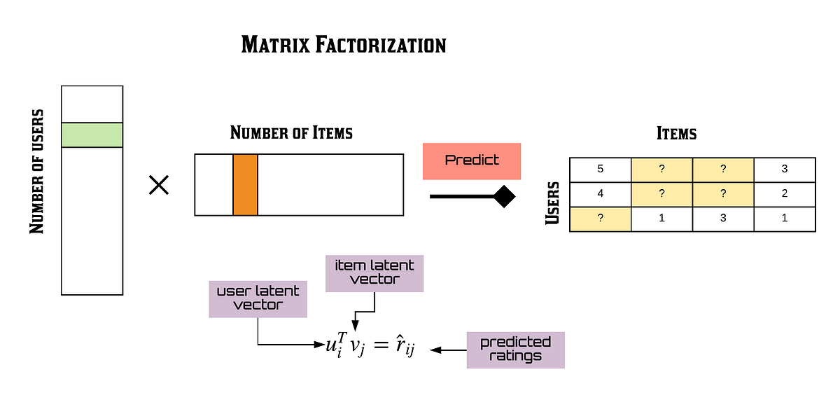
MF: Matrix factorization breaks a matrix into two latent matrices that when multiplied are supposed to recreate the original matrix. This is a form of matrix completion.

LRMC: This is again just matrix factorization as it’s referred to as low rank matrix completion.

NMF: This is nonnegative matrix factorization which just sets all negative values to zero as to not have negative values in imputation.

Gene Imputation:

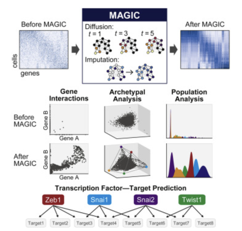
MAGIC: For genes, each cell is represented as a node in a graph with them connecting to other cells with similarity scores. Cells are then ordered out in space by a measure of distance. Missing or estimated cell values can then be estimated by neighboring cells to help denoise datasets.

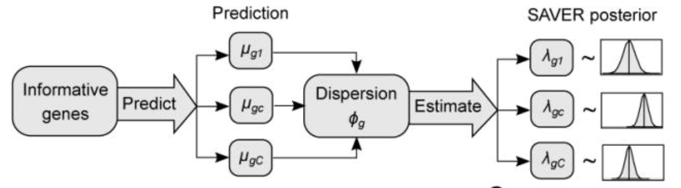
SAVER: For genes, existing relations are modeled using a poisson-gamma mixture. This distribution is then used to impute future values of an RNA sequence. Considered a better version of MAGIC.

VIPER: Variability-Preserving ImPutation for Expression Recovery (VIPER), is a technique for gene imputation that fits a standard lasso penalized linear regression model on both cell expressions and gene expressions. By doing both they can understand gene expression variability across cells after imputation.

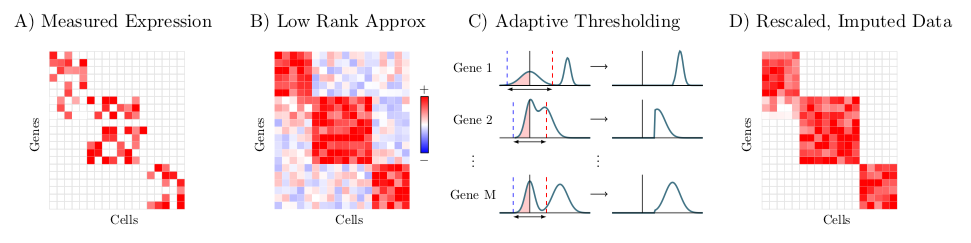
ALRA: For genes, ALRA is an imputation technique for genes that first uses a randomized SVD. Next each row is thresholded by the magnitude of the most negative value of that gene. Lastly the matrix is rescaled.

Time Series Imputation:

EWMA: Used for time series data, the exponentially weighted moving average (EWMA) gives more weight to newer data points and less to old ones. It isn’t now as commonly used. EWMAt=rt+(1-)EWMAt-1

TRMF: This is temporal regularized matrix factorization which is just matrix factorization specifically tailored to time series by capturing latent factors in multiple steps of a time series model, and then has the last row be a new row to have predicted.

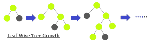
T-LGBM: Light gradient boosting machines (this one is specifically temporal) are used for time series data and are functionally similar to normal decision trees, except the nodes that are extended in this bagging technique are those with the most loss.

Complex Latent Model Imputation:

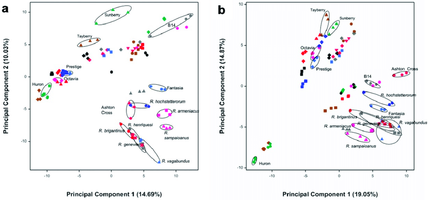
MIPCA: Multiple imputation in principal component analysis is used by first imputation multiple datasets using PCA. PCA is used by converting all data to new PC lines and then seeing where the data would fall on that line. This method overfits and doesn’t have any stochastic process for introducing noise, but due to the nature of multiple imputation it probably isn’t as bad.

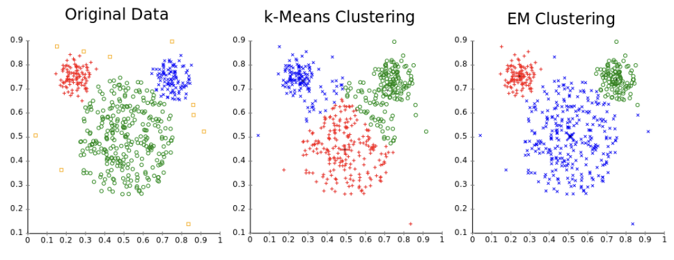
EM: Given a distribution, maximum likelihood estimation fits our data to that distribution, but it assumes multiple things, one being all data present is needed to make an accurate model. Given some variables are hidden, we use latent variables and sample over those instead. Estimation-Maximization estimates latent variables (step 1), and then maximizes parameters of a Gaussian Mixture Model to that new data (step 2). These two steps are repeated iteratively until an equilibrium is reached. It isn’t widely used and only seems useful in ensemble approaches. This can be thought of similarly to K-Means clustering.

RegEM: Numerical instability and convergence problems arise in EM in low data high dimensional datasets. This method in those situations recognizes it and implements regularization techniques.

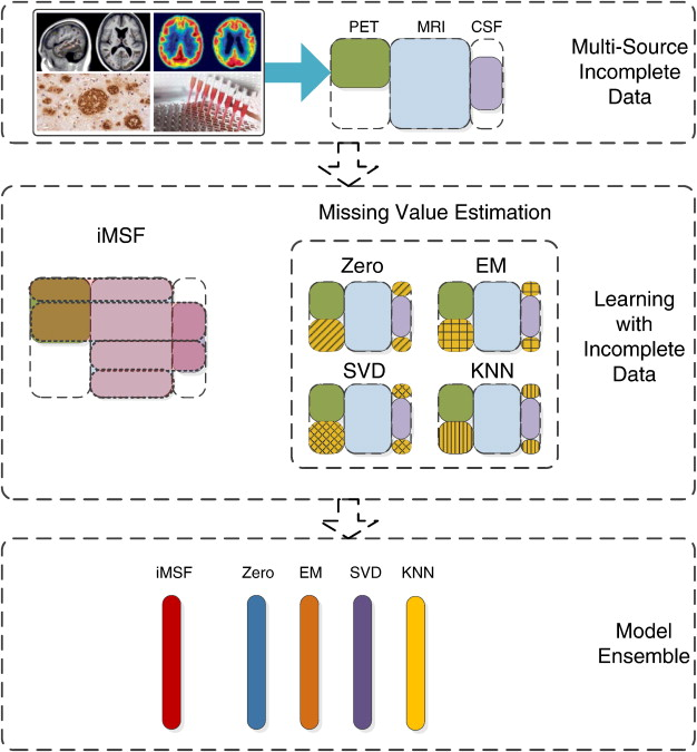
iMSF: Incomplete multi-source feature learning is an ensemble method that combines EM, SVD, KNN and a mean imputation method called “Zero”.

PPCA: To explain probabilistic PCA, we have to make a couple of steps:

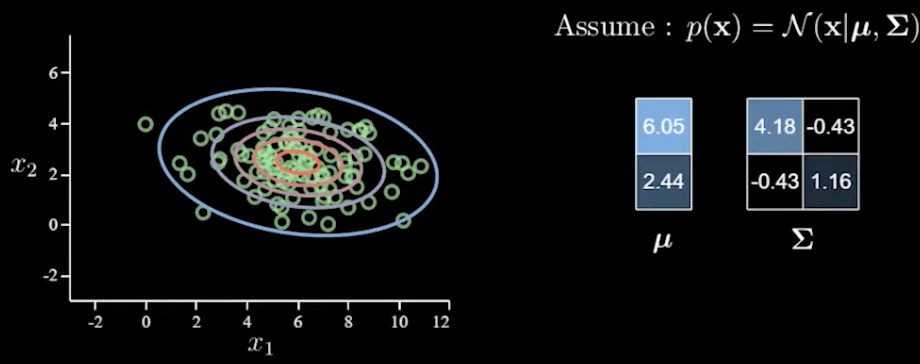
Multivariate Normals: Given a 2D graph with data points, a multivariate normal can be defined as p(x)=Norm(x|μ,Σ) where μ is a 2d mean vector and a covariance matrix Σ which is 2x2. With more and more variables given, the need for more parameters increases exponentially due to the covariance matrix growing too fast. This can also lead to overfitting.

Factor Analysis creates a loading matrix W of length L. x=Wz+μ+ε means our new value x is going to be equal to our latent space gaussian distribution value z we choose, a linear mapping W, plus a bias μ and noise ε.

\[p(z)=Norm(z|0,I), p(ε)=Norm(ε|0,Ѱ)\] \[p(x|z)=Norm(x|Wz+μ,Ѱ)\]

where μ is equal to the sample mean of x.

Optimizing this can be a pain, which is why PPCA is better.

Probabilistic Principal Component Analysis, or PPCA just has an easy to calculate closed form which I’m not going to delve into because I don’t want to write out and review eigen decomposition! 😛

What are the new-age techniques that are revolutionizing this space? Note that these new-age techniques all struggle to some degree with the required amount of data and compute in order to efficiently operate.

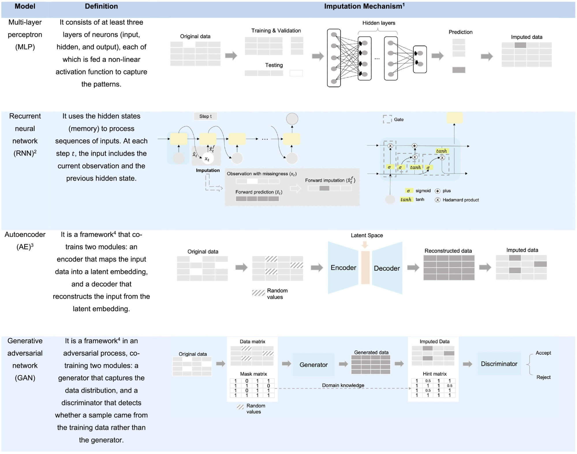
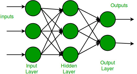
Multi-layer Perceptron (MLP) is a basic method consisting of at least three layers (input, hidden and output) used for the imputation process. MLPs (also known as NNs) are used in the remainder of methods but in differing ways, this way is just a very straight forward process of either a classification or a regressive value being assigned depending on the last layer’s usage of a softmax layer or a linear activation layer.

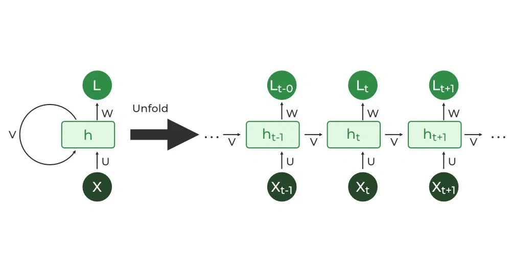
Recurrent Neural Networks (RNNs) are methods by which the same network is recurrently fed encoded information from a previous state. This then makes sense primarily in use-cases involving time series or signal data. At every new input a new output is guessed such that the value generated can be imputed in the data at hand. Other forms of RNNs include LSTMs, which are better but require more data, and GRUs which is a middle-ground in complexity between RNNs and LSTMs.

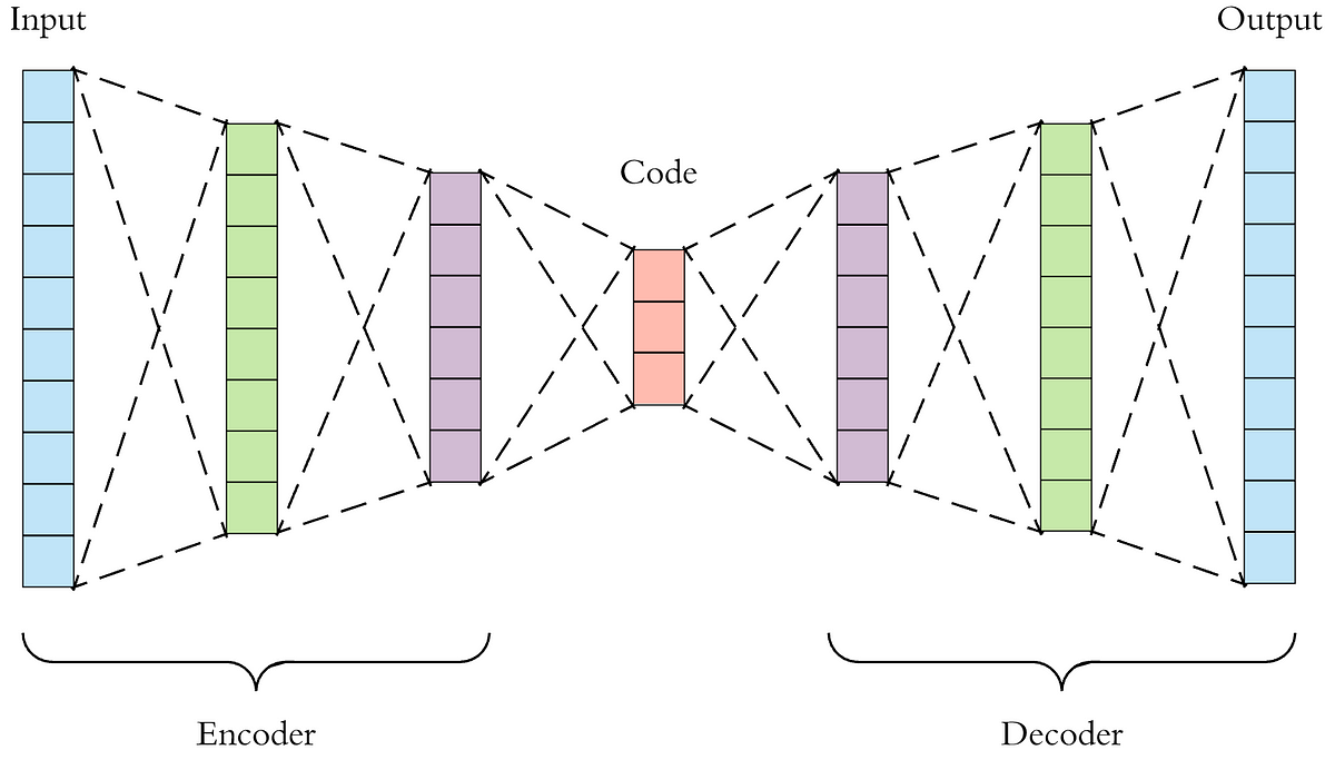
Autoencoders (AEs) are an interesting addition as their primary purpose is to encode data into a smaller version of oneself and to decode that data into a desired form. The pure form of an autoencoder is good at removing noise, however the specifically designed Denoising Autoencoders (DAEs) do a better job, as they train the AE to remove noise by injecting noise into the AE and train it to know what is noise and remove and impute data properly (noise in this case is missing data). Lastly, Variational Autoencoders (VAEs) train to recognize and shape areas within their encoded latent space in order to generate new samples by sampling from a distribution described by a mean and variance vector.

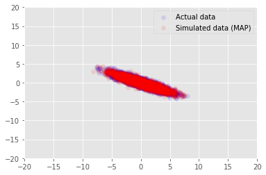
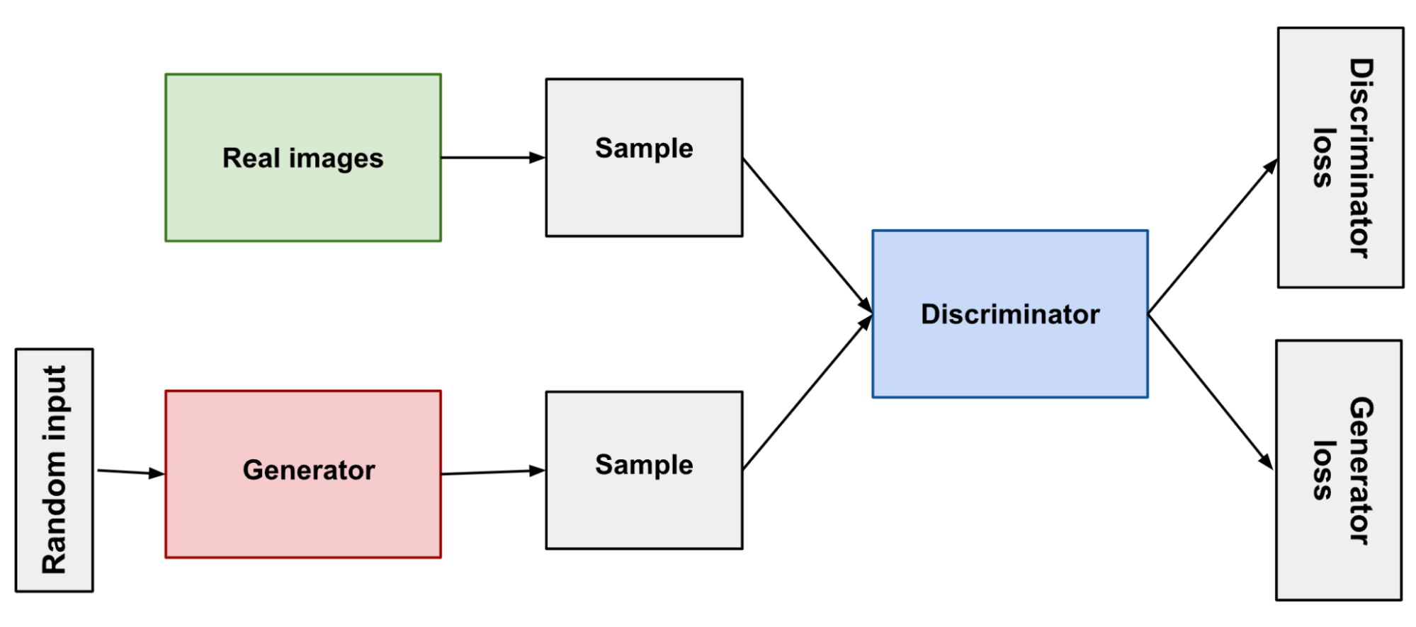
Generative Adversarial Networks (GANs) are a framework by which a generator tries to impute data and a discriminator that determines the difference between real and generated data. Similarly to VAEs, we can take a sample from a distribution to fill in the missing values.

In our understanding of imputation techniques there are two other important factors to consider. That is whether the imputation strategy has a separated imputation strategy, where the predicted value isn’t imputed as well, or an integrated imputation strategy, where the final result is also calculated using the same technique.

The other important factor is the data type in question. In health, we have tabular static data, tabular temporal data, genomic data, image data, signal data and multimodal data which combine any and all of the above. Now let’s look at which models were most widely used in each type of data!

Tabular Static Data:

12 autoencoder models, 10 MLP models and 5 GANs were used. Multiple data types for all methods require extra encoding and activation customization.

Tabular Temporal Data:

21 RNN models, 15 autoencoder models and 3 GANs were used.

Genomic Data:

9 autoencoder models, 4 MLP models and 2 GANs.

Image Data:

All 6 studies utilized GANs.

Signal Data:

What makes signal data different than that of tabular temporal data is that of a much higher frequency of sampling. 3 autoencoder models one GAN and RNN model were used.

Multimodal Data:

5 autoencoders were used, 2 MLPs and 2 RNNs were used. “The fusion of mode-specific models is essential when encoding multi-modal data.”

So what?

The paper says the methods of deep learning outweigh that of non-deep learning techniques. However a major problem is the lack of quality on the analysis of the underlying method in each paper. There are no papers brought up here that discuss how and why certain methods may fail, such as the instability of GANs and the lack of baselines they often have. Other analysis on how well these new DL models fundamentally learn statistical relationships is still in question, and when is the best time to correctly leverage these technologies. Not all papers saw that DL techniques performed better, and there was little to no analysis on the reasoning for this decision. Is there too little data in some cases? Are researchers properly implementing techniques?

There is room for a much better analysis of data imputation techniques and their practicality in health sciences.