The Theoretical Underpinnings to Analysis of Modern Multimodal Generative Latent Models
“How do we take in complicated data and accurately generate more of it?”
What motivates this post is an interest and desire to develop a keen understanding of how deep generative models work. From a theoretical to a practical analysis I want to be able to understand and explain these collections of models. This field is massive, and for my purposes I’ll be examining and walking through latent models. Latent models specialize in their ability to understand complex sources of data. My research involves the use of multimodal data to improve performance of generative models, so with this focus we can begin our adventure!
The manifold hypothesis states that all real-world expressions lie upon a smaller subset of data, that expresses itself in a higher dimensionality. This hypothesis underlies much of how machine learning works, and intuitively makes sense. When we imagine objects, our brain stores said objects in a collection of neurons, there exists this compression of information.
Let’s say we have a highly complex piece of data x, say a picture of a horse. We wish to compress said horse into a manifold. The representation that horse resides in is our latent space denoted as z.
What would the process be for not only learning how to represent a horse (autoencoder), but to also represent a distribution of horses? We want to represent horses, as well as all kinds of horses in a statistical manner. I find a lot of talk around this topic does the ground work of math first, and builds up to the bigger picture. I’m going to instead describe the bigger picture, and work my way down to the math such that we cultivate a better intuitive feeling for the math.
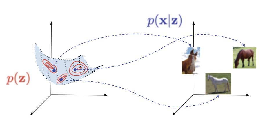
- We want to encode some x into a latent space z. The probability density function (pdf) of this is “p(z|x)”. (A pdf is just a function of probability over a space. So over a discrete space of a coin flip, tails is 0.5 and heads is 0.5. Over a continuous space, we find that calculating the probability at any given space is hard, unless we’re dealing with very specific functions be it gaussian or poisson distributions.)
- We want to sample from said latent space z, such that we get a sampling away from out simple sample. The pdf of this is “p(z)”.
- We want to decode that sample into a new x’. The pdf of this is “p(x’|z)”.
- We want to tweak our encoding and decoding process to not only represent x’, but to represent the distribution that x’ comes from.
Now…
- Encode a value to a mean and covariance matrix: \(x \rightarrow \mu(x), \Sigma(x)\)
- Calculate a sample: \(z = \mu(x) + \Sigma(x) \cdot \epsilon \text{, where } \epsilon \sim \mathcal{N}(0, 1)\)
- Decode \(z \rightarrow p(x\vert z)\)
- Optimize the process, taking into consideration how well the VAE can create horses, as well as deviate from the mean horse in a proper manner. We are optimizing some parameters given an input x and a chosen prior z.
Let’s focus on this last step and how we derive a suitable formula. We know our final optimization must take into consideration both reconstruction and statistical representation, and we know we can only do this using values we have. Theoretical values we don’t have, for instance, is the perfect encoding p(x|z). We don’t know what the ideal distribution is p(z) in a latent space and instead resort to using a gaussian distribution N(0, 1). So let’s start from the beginning and finally derive this equation and see why it makes sense!
The below equation is our starting point that describes how the probability of x is the probability of x given all distributions z. Understanding what the actual latent distribution is for z isn’t tractable, or isn’t really easily calculable. Instead we’ll come up with neat substitutions down the road!
\[p(x) = \int p(x|z)d(z)dz\]Let’s first multiply each side by the natural log, as to simplify our calculation eventually to a summation.
\[ln(p(x)) = ln \int p(x|z)p(z)dz\]We also know that we don’t have the exact distribution p(z) that perfectly maps onto our latent space, so we’ll instead use a tractable distribution q(z). This borrows from variational bayesian methods which look to provide an approximation of a previously intractable distribution. For now, just imagine we’ll sloppily use the normal distribution N(0, 1) for q(z).
\[ln(p(x)) = ln \int \frac{q(z)}{q(z)} p(x|z)p(z)dz\] \[ln(p(x)) = ln \mathbb{E}_{q(z|x)}[\frac{p(x|z)p(z)}{q(z)}] \text{, where }\ \mathbb{E} _{q(z|x)} = \int f(z)q(z)dz\]We have to move this natural log inside of our expectation, which we can only do with Jensen’s Inequality. Jensen’s Inequality is used in this case to show that we cannot perfectly optimize this problem, but rather come to an approximation.
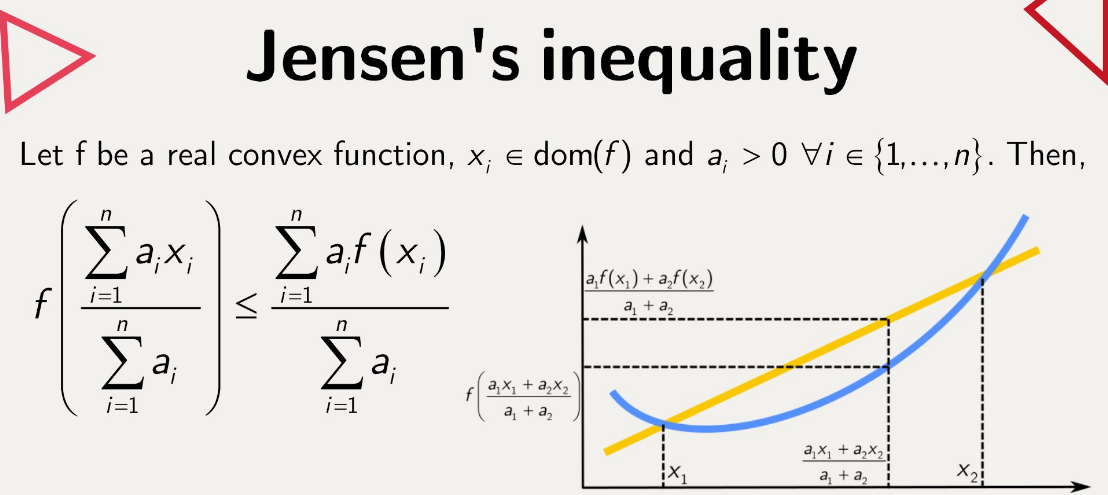
Jensen’s inequality does mean that we lose some specificity in our approximations, however consider that our optimization landscape may actually become easier and less noisy, and there’s research to show that getting as close to the lower bound of error in estimating our distributions may not actually give us the best results.
\[ln(p(x)) \geq \mathbb{E}_{q(z|x)}[\frac{p(x|z)p(z)}{q(z)}]\] \[ln(p(x)) \geq \mathbb{E}_{q(z|x)}[ln(p(x|z)) + ln(p(z)) - ln(q(z))]\] \[ln(p(x)) \geq \mathbb{E} _{q(z|x)}[ln(p(x|z))] - \mathbb{E} _{q(z|x)}[ln((q(z)) - ln(p(z))]\]This equation is known as our Estimated Lower BOund (ELBO). Let’s take a step back from this complex formula that isn’t intuitive and think about what exactly we’d want in a formula for generating statistically representative samples. Well, we’d want a term to punish how accurate the final result. The second term we’d want is one that enforced the statistical distribution we’re looking for. We’re basically desiring a mix between complete recreation accuracy and the variation that we desire in a generative model. This is exactly what we end up with! Let’s take a look.
Our first term is the log likelihood of how well our decoder recreates our data x from our latent data z. Our second term is the Kullback Leibler Divergence (KLD) equation, in which the statistical distance between one probability distribution from another. Our two distribution is the one we create compared to the one we desired.
\[\mathbb{E} _{q(z|x)}[ln((q(z)) - ln(p(z))] = \text{D} _{\text{KL}}(q(z)\parallel p(z)) = \sum _{Z \epsilon z} q(z) log(\frac{q(z)}{p(z)})\]Here we’re summing up the ratios multiplied by q(z) to find the surprise of how close our distributions align. This way we can enforce how well our model fits the distribution!
\[\text{Log Loss} \geq \text{Reconstruction Error} + \text{Statistical Distribution Error}\]The log of p(x|z) we take the natural log of the pdf of a gaussian distribution
\[\text{Reconstruction Error} = \text{MSE}(x, x') = \sum^{n}_{i=1}\frac{(x _{i} - x' _{i})^{2}}{n}\]To find out the KLD equation for easily comparing a diagonal multivariate normal to a standard normal distribution I looked it up on wikipedia and found this equation haha.
\[\text{Statistical Distribution Error} = D_{KL}(\mathcal{N}(\mu(x), \sigma(x)) \parallel \mathcal{N}(0, I)) = \frac{1}{2} \sum^{n} _{i=1}(\sigma^{2} _{i} + \mu^{2} _{i} - 1 - \text{ln}(\sigma^{2} _{i}))\]In our code now, we’ll take an image x, encode it to two separate vectors μ and σ in our latent space. We’ll sample from said latent space z = μ + σ * N(0, I). From this z, we pass it into our decoder and get x’. Then we plug in our values (x, x’, μ, σ) into our equation and get a loss to then optimize our parameters for.
\[\text{Log Loss} \geq \sum^{n}_{i=1}\frac{(x _{i} - x' _{i})^{2}}{n} + \frac{1}{2} \sum^{n} _{i=1}(\sigma^{2} _{i} + \mu^{2} _{i} - 1 - \text{ln}(\sigma^{2} _{i}))\]I hope this equation makes sense now and where and why we use it!
Potential Issues
Posterior collapse could occur where the proper representation doesn’t exist because the encoder and decoder are too powerful. All deviations in our latent space are instead treated as noise and there’s no meaningful distinction in our sampling of z.
The Hole Problem is where there is a mismatch between the areas the prior thinks are high probability and that of the posterior encoder think are high probability.
The out-of-distribution problem talks about the difficulties of how a model can understand data it’s train on, but then cannot properly generalize or recognize new data from a different, new distribution.
Improving Our Model
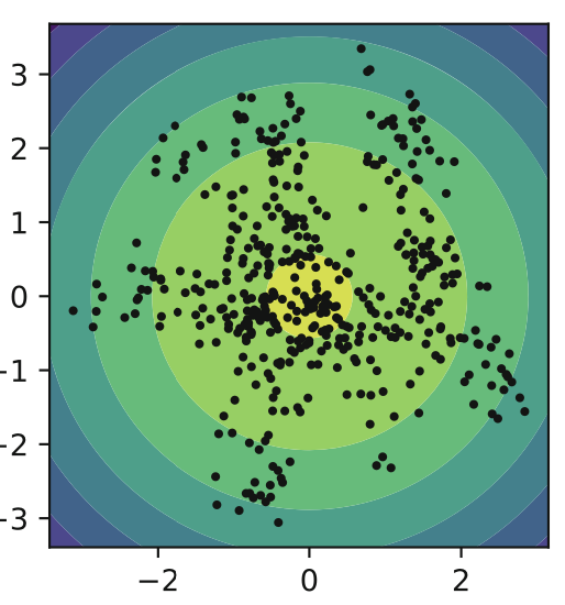
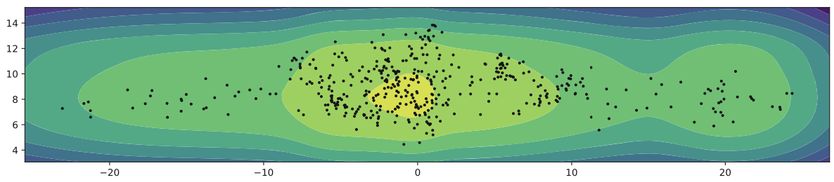
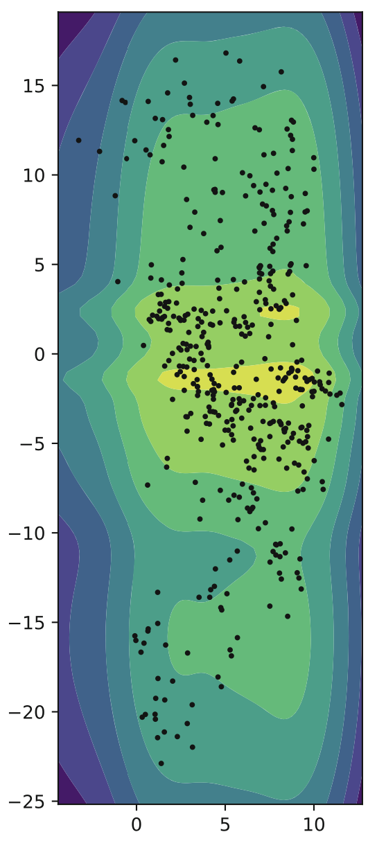
As mentioned before, if there’s a big mismatch between the aggregated posterior and the prior, we won’t be able to represent data properly. Encoding a VAE into a 2d space and filling in the spaces we can see that some areas aren’t used by the encoder. This is that mismatch. Instead we can use a Mixture of Gaussians (MoG) prior to better fit the data.
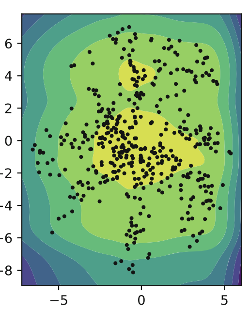
An improvement upon MoG was that of VampPrior: Variational Mixture of Posterior Prior. In the equation below u is a set of trainable parameters that are randomly initialized and trained via backpropagation. What we’re doing is using different density estimators to map onto our low-dimensional latent space.
General Topographic Mapping (GTM) defines a grid of K points in a low-dimensional space similar to a sheet a paper that we then scrunching up and wrinkling it to better fit the densities of our actual distribution. We can even combine GTM and VampPrior to get even more complex fits! But remember that complexity isn’t always better, as we risk overfitting.
Flows
One promising area that has recently gained popularity is that of flow-VAEs. Let’s say we want to model some complex probability distribution. One way of doing so is doing a series of simple transformations on a simple Gaussian until the result roughly approximates our desired probability distribution. Let f be a series of invertible transformations, resulting in a final bijective transformation where every input has exactly one output.
Figuring out the density seems easy. We just use the inverse. However the inverse doesn’t take into consideration that our probability density should integrate to 1.
\[p(x) = p( \mathcal{f}^{-1}(x)) \begin{vmatrix} \text{det} (\frac{\partial \mathcal{f}^{-1}(x)}{\partial x}) \end{vmatrix}\]The inverse transformation is multiplied by the inverse jacobian determinant. This makes sense given the definition of a jacobian determinant is a scaling factor between one coordinate space and another. We are swapping coordinate systems and need to compensate for the change in density. We do this by mapping out the changes (jacobian), and then finding how much those scale the coordinate system (determinant).
You can probably tell by now, estimating a complex distribution through transformations is incredibly valuable in our latent dimension for variational autoencoders! This is the last prior we examine here, that of a flow-based prior.
Flows were originally used given the image input x, but this was computationally very expensive. Using them on a smaller latent space is much more efficient, and similar to GTM-VampPrior, the hyperparameters should be used to limit the model, as otherwise it may overfit the data.
There is also more theory regarding different types of flows and how to arrive at them, but for the sake of brevity in an already incredibly long post, let’s skip this haha.
From the top!
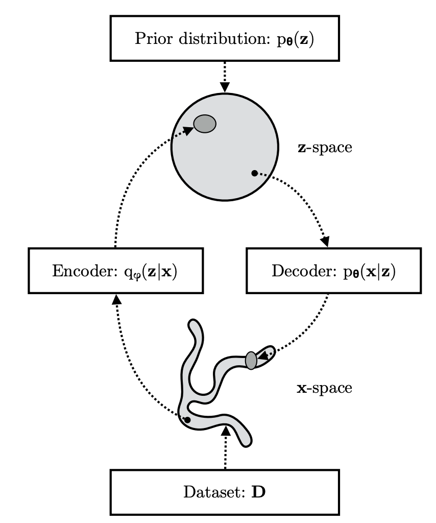
We’re taking a complex distribution p(x) and approximating it using ELBO. This image shows this process succinctly, and later we’ll dive into real world applications of this latent space visually for extra clarity.
One important note is that of the use theta θ and phi φ symbols used in this image, and well, everywhere else in this field. Remember how we’re optimizing a neural network? Well, the parameters for that network is referred to as θ, where our input vector x and prior z are simply inputs into the optimization problem! φ then refers the our prior’s parameters that can also be parameterized. Now, given a regular vanilla VAE that outputs a categorical distribution is the following:
\[q _{\phi}(z|x) = \mathcal{N}(z|\mu _{\phi}(x), \sigma _{\phi}^{2}(x))\] \[p(z) = \mathcal{N} (z|0, \text{I})\] \[p _{\theta}(x|z) = \text{Categorical}(x| \theta (z))\]“But the usage of theta and phi are opposite of the picture above!!” Yes… there isn’t a consensus among everyone what symbols to use for what. And yes it can makes things confusing haha. Ultimately it’s just a little symbol people put onto their equations to make the equation look scarier. Unless it’s written as a true optimization problem such as the following:
\[\theta \leftarrow \text{arg}\max_{\theta} \frac{1}{N} \sum _{i} \log p(x _{i})\]This means for custom priors we can also construct optimization equations for their own parameters and backpropagate appropriately.
One last note is something referred to as the reparameterization trick. When we backpropagate we have to assign reward or blame to different weights for how much they were right or wrong. We can’t do this well when we change one of our values σ via a stochastic process because the equation is no longer differentiable. So instead we construct our code to have a calculated μ and σ and then add an error term N(0, 1) that’s multiplied by our σ. This way we can appropriately backpropagate and our stochastic process is properly written off as noise.
Where Do We Go From Here?
This is a hard question. In the rapid world of ML, finding what works best may change one year to another. With a constantly developing assortment of architectures, terminology and metrics to test with, what may seem impossible one day is trivial the next. Let’s get a better grasp of recent developments related to what we originally came here to find, we’re here for statistically-aware multimodal imputation after all! We can go down every rabbit hole, but we must focus on our main pursuit!
(2017) Multi-stage Diagnosis of Alzheimer’s Disease with Incomplete Multimodal Data via Multi-task Deep Learning
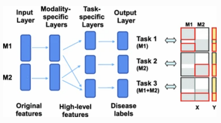
This method was covered in a previous post. Essentially we process each modality separately, send the data to another layer that matches all inputs given, and then we predict the final outcome.
Training is tricky, as training the initial modality layer for each task will change the layer in ways that don’t effectively train every task the same, so we play a game of “catch up” here. We constantly freeze various networks in training certain tasks, only for whatever was trained to then perform differently on other tasks that weren’t updated.
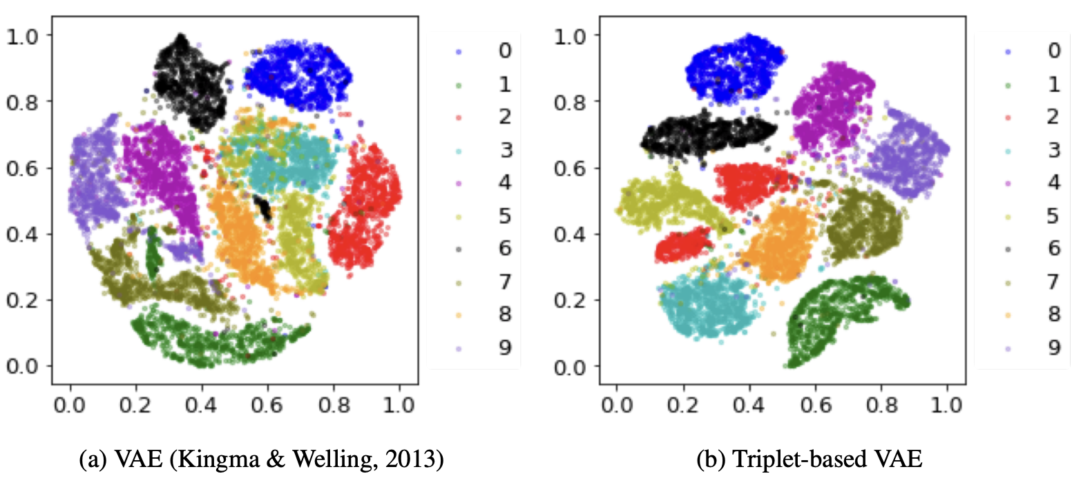
(2018) TVAE: Triplet-Based Variational Autoencoder Using Metric Learning
This is a standard VAE architecture however we add an additional loss term.
We select three samples. The first is the anchor, the second is a value close to the anchor, and the third is a sample further away from the anchor. We then add a loss metric to our model where if the latent space between the two similar means are further away than the latent space between the two dissimilar means, then punish the model. This way we are encouraging samples that are similar in value to have similar latent values as well.
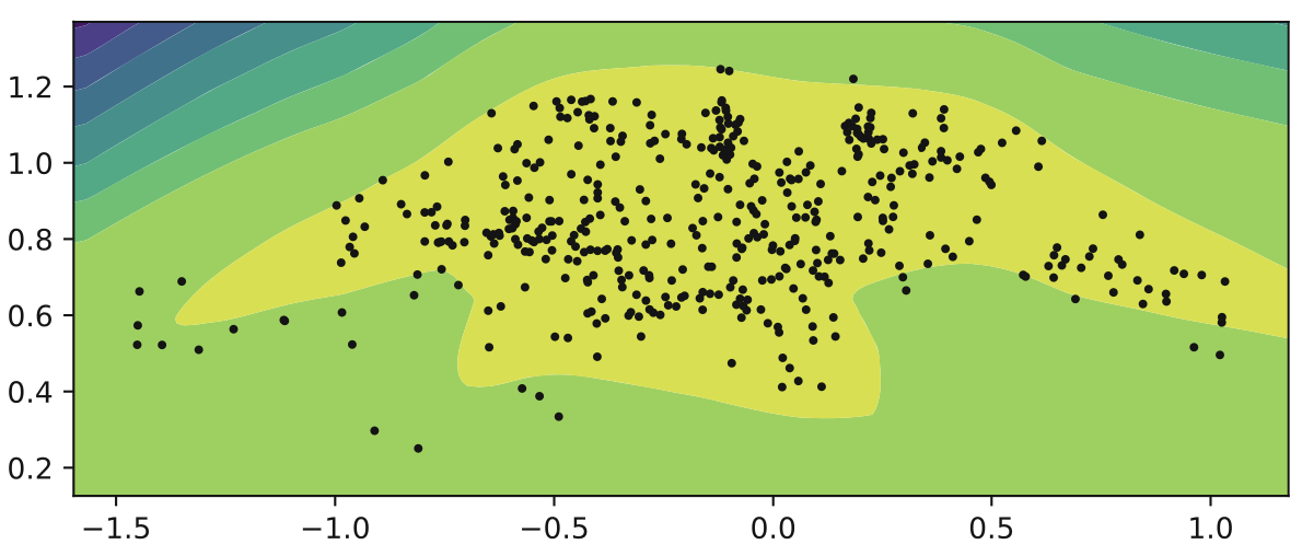
\[L _{vae} = L _{rec} + L _{kl} + L _{triplet}\] \[L _{triplet}(x _{a}, x _{p}, x _{n}) = \max {0, D(x _{a}, x _{p} - D(x _{a}, x _{n}) + m}\]Where the different x values refer to anchor, positive and negative respectively. This model improves the VAE accuracy on the MNIST dataset from 75.08% to 95.60%! Also look below at our latent gaussian circle and how much clearer the model becomes! Beautiful.
TabDDPM: Modelling Tabular Data With Diffusion Models
A little bit on diffusion models. We have the entire model in a first order markovian chain that deconstructs and reconstructs data. The forward process gradually adds noise to the initial sample. The reverse diffusion process gradually denoises a latent variable. Similarly to our equation before, we just add multiple latent encoding and decoding models that chain together to dissemble and create images.
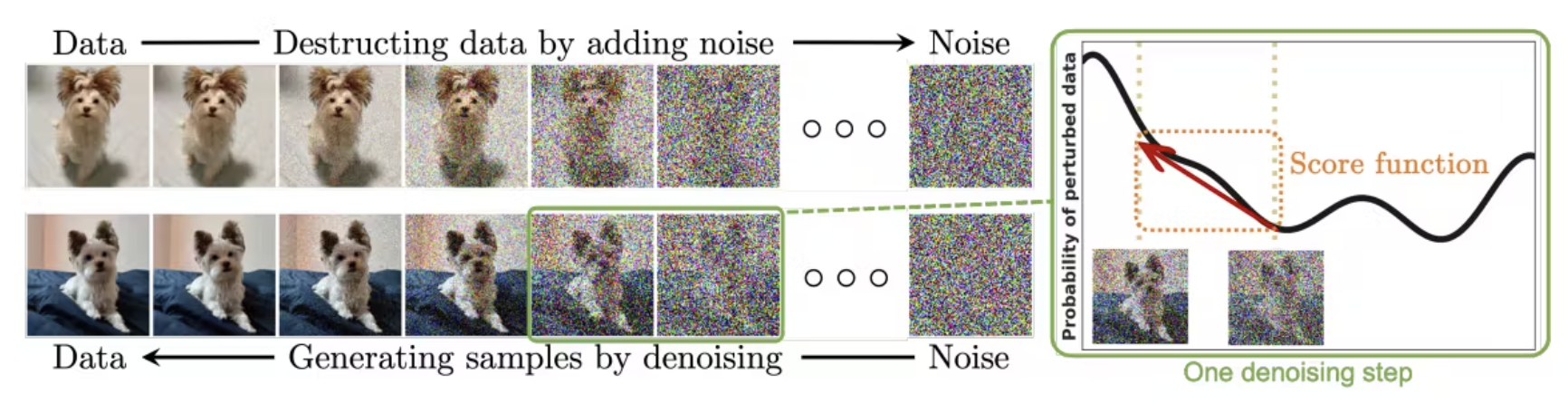
This is similar to our VAE equation, however we’re accounting for multiple layers T that each add or remove noise! We have a forward process q and a diffusion process p:
\[q(x _{1:T} \vert x _{}0) = \prod^{T} _{t=1} q(x _{t} \vert x _{t-1})\] \[p(x _{0:T} = \prod^{T} _{t=1} p(x _{t-1} \vert x _{t})\] \[\log q(x _{0}) \geq \mathbb{E} _{q(x _{0})}[\log p _{\theta} (x _{0} \vert x _{1} - \text{KL}(q(x _{T} \vert x _{0}) \vert q(x _{T})) - \sum^{T} _{t=2} \text{KL} (q(x _{t-1} \vert x _{t}, x _{0}) \vert p _{\theta} (x _{t-1} \vert x _{t}))]\]Note that our work deals with heterogeneous data and traditionally small sample sizes of tabular and/or image data. We’ll find a solution to that by looking at how we replace our traditional gaussian distributions with categorical distributions.
Gaussian:
\[q(x _{t} \vert x _{t-1} := \mathcal{N}(x _{t} ; \sqrt{1 - \mathcal{B} _{t} * x _{t-1}, \mathcal{B} * \text{I}}))\] \[q(x _{T}) := \mathcal{N}(x _{T}; 0, \text{I})\] \[p _{\theta}(x _{t-1} \vert x _{t}) := \mathcal{N}(x _{t-1} ; \mu _{\theta} (x _{t}, t), \Sigma _{\theta} (x _{t}, t))\]Where Β is a constant along with α such that:
\[\alpha _{t} := 1 - \mathcal{B} _{t}\] \[\mu _{\theta} (x _{t}, t) = \frac{1}{\sqrt(\alpha _{t})}(x _{t} - \frac{\mathcal{B} _{t}}{\sqrt{1 - \alpha _{t}}} \epsilon _{\theta} (x _{t}, t))\]These constants are needed for the model to understand the “groundtruth” noise component ε. Now, for multinomial diffusion models we’ll see the similarities and understand what is going on on viewing the formulas:
\[q(x _{t} \vert x _{t-1} := \text{Cat}(x _{t};(1 - \mathcal{B} _{t}) x _{t-1} + \frac{\mathcal{B} _{t}}{\text{K}})\] \[q(x _{T}) := \text{Cat}(x _{T}; \frac{1}{K})\] \[p _{\theta}(x _{t} \vert x _{0}) := \text{Cat} (x _{t}; \alpha _{t} x _{0} + frac{(1 - \alpha _{t})}{K})\]There’s more, but this enough shows how we’re replacing the distributions with ones that better match solving for binary and categorical data. But what if we’re not solving for those types? Well then we simply use a regular diffusion model!
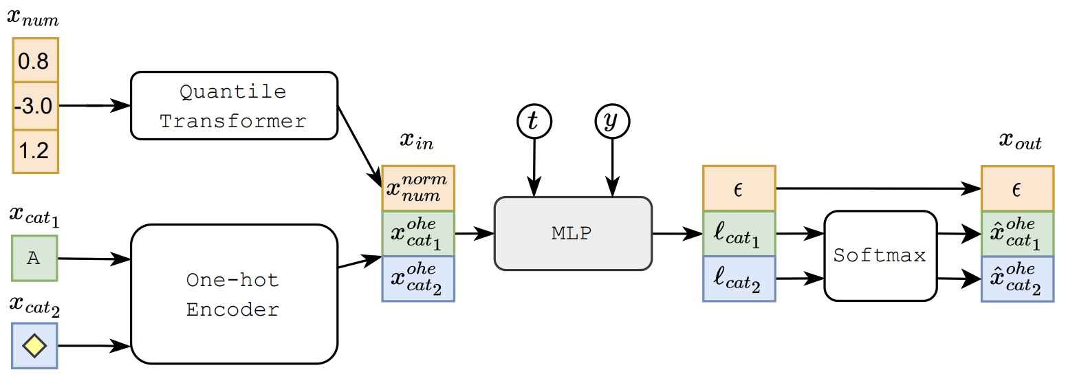
One really cool part here is that we make use of a gaussian quantile transformer such that when we’re diffusing data we get results that can better match our gaussian diffusion model priors! The results of this model are really good and beat other models, but the models they compare to are GANs which aren’t necessarily competitive in tabular data generation. It’s hard to say, because there’s no baseline comparison to traditional methods such as KNN, or even mean imputation. This makes measuring results unsatisfying, but there is also a point of intrigue for what can be done in the future using this technology that has dominated visual data generation. Maybe there can be a mutlimodal diffusion model that can easily build off of this existing technology 🤔🤔🤔.
(2022) Tabular data imputation: quality over quantity
The algorithm used is called kNNxKDE which is a hybrid method of kNN for conditional density estimation (KDE). This has a worse RMSE, but a better log-likelihood, which makes sense given we’re trading off locational error for dataset structural consistency. It’s an interesting paper that keeps us sharp on what metrics really matter.
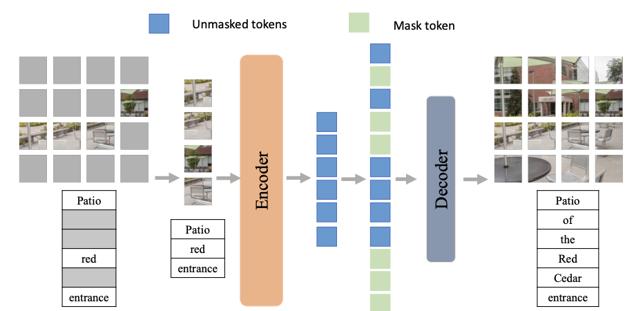
(2022) Multimodal Masked Autoencoders Learn Transferable Representations
I won’t spend much time with this because it doesn’t deal with tabular data, which can have a huge effect. But it’s an important architecture that comes up a lot in effective training cases. The architecture and result doesn’t seem quite powerful enough given this is a 2022 paper. Note it’s still a good paper, and I’ve read plenty of papers I chose not to include because the results were dubious with little depth or substance. This paper in contrast still showed good results.
(2022) Explainable Dynamic Multimodal Variational Autoencoder for the Prediction of Patients With Suspected Central Precocious Puberty
This paper I originally looked at and loved. It’s more complex but has promising theory behind it. We’re essentially taking many VAEs that each encode their own μ and σ.
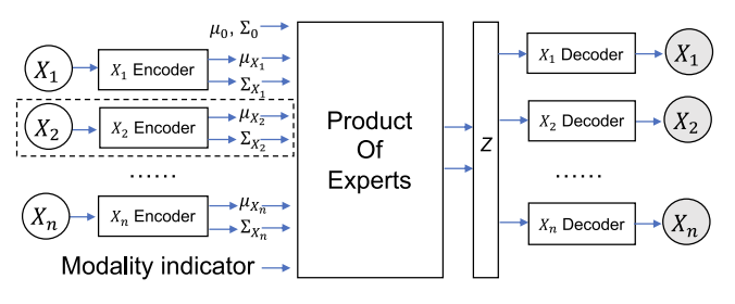
What we do is we encode every modality separately to a common latent space where we can then find the overlap of distributions and sample from that distribution instead. How do we handle image data? Well… the authors seem as though they conducted manual feature extraction to ultimately pass in all tabular data in the end. This isn’t great, but extending off of this work to include latent features derived from transfer learning seems promising.
This paper uses the following definition of our ELBO optimization function:
\[L _{ELBO}(X) = -\alpha D _{KL}[q _{\phi}(z \vert X) \vert p(z)] + \mathbb{E} _{q _{\phi (z \vert X}}[ \sum _{X _{i} \in X} \mathcal{B} _{i} \log p _{\theta} (X _{i} \vert z)]\]It’s written a little differently, but almost means the same thing. One thing that’s added are the terms beta and alpha which are used as weights. The authors don’t go into how these weights are applied or adjusted, so we have to assume manually in a hyperparameter grid search of some sort. This means that how much punishment is doled out to recreating a distribution versus recreating the original image is changeable. Another model that does this is a BVAE which basically just introduces these terms as a standalone model to demonstrate that real world performance doesn’t alway match up to mathematical theoretical equations.
Another thing about this loss function is the summation of recreation loss among all modalities in the set of X referring to each modality available. To make up for the lack of information regarding image data (X and US are the names of the modality images) that had to be manually entered, the loss function for each modality looks like the following:
\[L _{DMVAE}(X, M) = L _{ELBO}(X, M) + L _{ELBO}(X _{X}, M) + L _{ELBO} (X _{US}, M)\]Honestly this whole paper is a lot of fuss and extra work for only a 0.1+ improvement. VAEs were at 0.89 AUROC (I doubt optimized), and this method, they call DMVAE scores 0.90 AUROC. The F1 scores were 0.8057 for the VAE and 0.8152 for the DMVAE. It’s an improvement, and maybe we’ve just reached the level of knowledge possible given the problem at hand; we’ll never hit 100% accuracy.
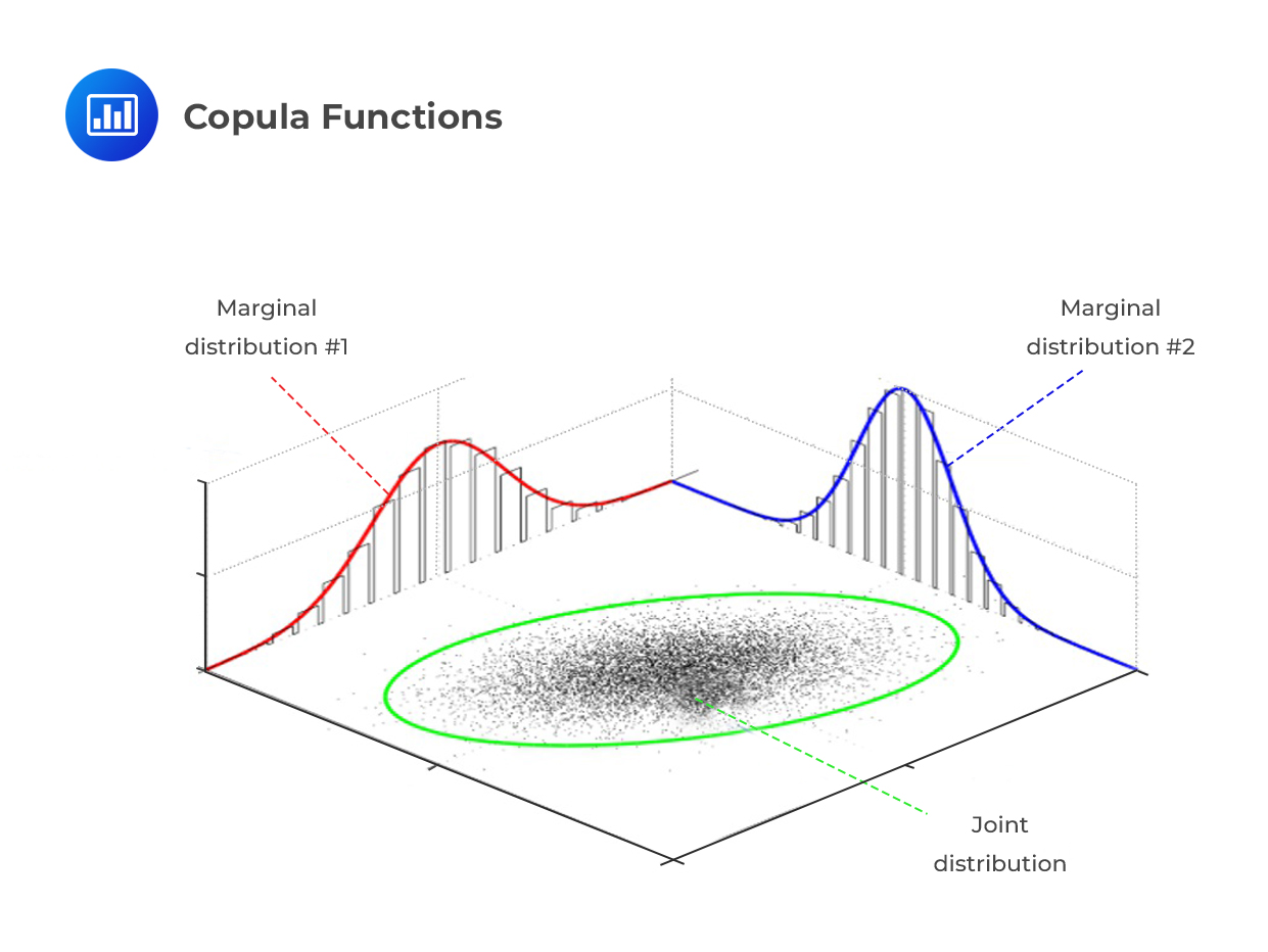
(2023) Comparison of tabular synthetic data generation techniques using propensity and cluster log metric
This paper looks at varying techniques for generating tabular data. This paper is an amazing baseline paper for our future comparisons in multimodal models. CART is the best performing model. This is a complex and malleable decision tree similar to miss forest. Copulas performed second best. Gaussian copulas transform all variables to a gaussian. Then it models the reliance of other variables on each other to create a covariance matrix to sample from. Our TVAE model performed third best. We already covered this method!
The metrics were based on log cluster and propensity. However, the quality of maintaining correlations was not tested.
One interesting fact was that of how poorly GANs performed. Remember that promising diffusion model earlier? Until there are proper comparisons among these models, this paper shows GANs are not necessarily a good investment for any practicioner looking to impute data, especially given the best model here, CART is a simplistic decision tree while diffusion models are incredibly complex and show no real benefit yet. I am suspect that other papers show improvements over tree-based methods. It could be that optimal parameters weren’t reached, my post “We Don’t Push ML To Its Limits” talks about this trend in academia. It could however be that most other implementations of tree-based methods just chose the improper Miss Forest compared to CART, and that CART is a real gem, though looking through the model, it doesn’t seem capable of high quality data generation at a larger scale than what was tested for. It’ll be interesting to see how it compares to other architectures and datasets in the futrue!
In Conclusion
Our original desire was to seek how multimodal data is used for the purpose of tabular imputation, and we didn’t really see anything worthwhile here. A lot of topics talk around this subject, but there’s a hole in the literature for quality research to come through and make a meaningful prediction.
As for latent model generation, we went into great deal on how VAEs work, and a little on how diffusion models work (better for a completely different blog due to their complexity). Nonetheless, the theory practiced here, as shown in our little coverage of diffusion models, carries over to other generative models as well.
This field is quite interesting, and I’m super excited to learn more and contribute to such an amazing body of literature!