How Multimodal Transformers Work For A Medical Usecase

Transformers From The Bottom Up

While previous AI technologies proved useful in the past, the power of the transformer has been unmatched in every regard. But how does it work? What is its purpose? For our purpose of healthcare, how can this be applied to help people? Let’s go back to the inception of the transformer, and slowly build it out to the more complex implementations of today.

The original designers of the transformer wanted to process words, and translate them to another language. Previously this had always been a sequential task, where we have to rely on a memory cell of sorts to keep track of what was said previously. Every word is a pain point that needs to be processed iteratively with no easy parallelization. Attention is the idea that we may be able to look at an entire sentence and have a neural network analyze every connection and decide which words are relevant to other words.

Transformer Overview

1. Randomly sample a block of data repeatedly. Each block will be of size T (time). Once we’ve collected enough samples we’ll form a batch of tensors of size (B, T).
2. Embed each word into a numbered value through an embedding table. The embedding is now (B, T, C). This conversion is a neural network layer that is trainable, and in this case is learning how to best represent words in a higher dimensional space. Then we will concatenate said embedding with a position embedding table such that our model will understand how words are in relation to others.

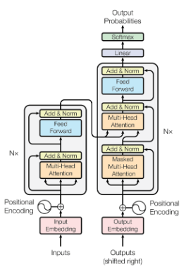
   self.token_embedding_table = nn.Embedding(vocab_size, n_embed)
   self.position_embedding_table = nn.Embedding(block_size, n_embed)
   

3. Next we pass our data into a series of blocks. Each block consists of the MultiHeadAttention mechanism followed by a simple neural network feed forward layer.

self.sa = MultiHeadAttention(n_head, head_size)
self.ffwd = FeedForward(n_embd)
ln1, ln2 = nn.LayerNorm(n_embd)
x = x + self.sa(self.ln1(x))
x = x + self.ffwd(self.ln2(x))

Ok…

Let’s take a step back. We skipped over the most important part being the inner workings of the block! Here is where we can appropriately see how we’re not just learning from a sequence of characters, but doing so in an easily parallelizable way. Previously we’ve had to iteratively process each step in a sequence, guess the next piece and so on, but here we’ll process all steps simultaneously. We then create a network that allows for some pieces of information to be more relevant to other pieces of information. In the context of language, an adjective will generally always be tied to a noun, so highlighting the relevance of a descriptor to a specific noun will provide a greater understanding to the network itself.

Block Overview

Going back to our block:

self.sa = MultiHeadAttention(n_head, head_size)
self.ffwd = FeedForward(n_embd)
ln1, ln2 = nn.LayerNorm(n_embd)
x = x + self.sa(self.ln1(x))
x = x + self.ffwd(self.ln2(x))

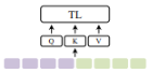
Given we’re working with sentences for the purpose of language translation as set out in the original paper, we want to come up with a way to attach the meaning of a noun to its adjectives. Each word conducts a query, and looks for keys to match their meaning. A noun like “cat” is matched to “black”, especially when the two words are in the proper position. So our query matrix is identifying if what we’re looking at is a noun, and a key is looking to match a query vector, like a response. Every word is then sending out a “Who matches with me?” query matrix embedding, as well as a “I’m looking for this type of embedding” key matrix embedding. The query embedding “cat” finds the query embedding “black”, and are optimized such that when they multiply together, they indicate a match by being close to 1 and further away from 0. A dot product is simply done, where all query and key embeddings are matched up against each other and this way, we have which queries and keys have high attention.

self.key = nn.Linear(n_embd, head_size)
self.query = nn.Linear(n_embd, head_size)

k = self.key(x)
q = self.query(x)

wei = q @ k.transpose(-2, -1) * k.shape[-1]**-0.5

If we wanted to translate from one language to another we can change our “self-attention” to a “cross-attention” architecture by referring key and query maps to two different inputs.

k = self.key(x_english_embedding)
q = self.key(x_chinese_embedding)

The variable “wei” refers to the attention weights. Here we have the dot product using @, however we also have k.shape[-1]**-0.5 which is unexpected. This here is simply a scaling factor used to control the values of dot products from becoming too large in higher dimensions. Remember that we’re also looking at instances in which we are trying to predict the next value. We must then hide future values by using the next line:

wei = wei.masked_fill(self.tril[:T, :T] == 0, float('-inf'))

Next we apply a softmax such that each column adds up to 1. We’ll also implement a dropout to increase generalizability.

wei = F.softmax(wei, dim=-1)
wei = self.dropout(wei)

We currently have a weighting, so now we just need to know where in our embedding space to move our original embedding. If we had cat, and we want to move the embedding closer to black cat syntactically, we have to utilize a third linear network called “values”.

self.value = nn.Linear(n_embed, head_size)
v = self.value(x)
final_output = wei @ v

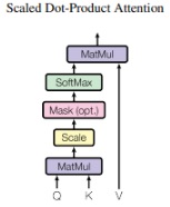
This entire step can be summarized by the equation

\[Z=SA(Q,K,V)=Softmax(\frac{QK^T}{\sqrt{d_{q}}})V\]

With the final_output, we add it to our original embedding to move said embedding closer to its actual meaning.

self.sa = MultiHeadAttention(n_head, head_size)
self.ffwd = FeedForward(n_embd)
ln1, ln2 = nn.LayerNorm(n_embd)
x = x + self.sa(self.ln1(x))
x = x + self.ffwd(self.ln2(x))

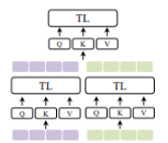
What is this MultiHeadAttention? We only looked at a single attention operation? Well the idea is that we can run multiple instances of this algorithm all at once, thus creating many “heads” by which can all be summed up with different keys, queries, values and embeddings. This allows for a more nuanced, robust system.

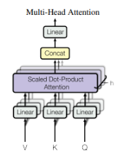
self.heads = nn.ModuleList([Head(head_size) for _ in range(num_heads)])

Each block has a multihead attention architecture that can then be run multiple times iteratively to encode deeper understandings of words. We may have a name of a person, who through the context of other words gives meaning. The name “Alex” may be referenced, but only in the context of Macedonian history or military conquests are we referring to “Alexander the Great”. The iterative environment allows for nuanced encodings to occur.

The Future is Multimodal

Transformers have an incredible ability to find patterns, even among varying sizes and types of data to the point that it may trivialize other previously very complex algorithms. Complex algorithms that specialize in specific tasks could get blown out by simple transformers due to the sheer power that transformers bring. The performance increases are massive, but do eventually fall off, and these models have a lot of parameters, meaning that we have to train on significantly more data to achieve the desired results. But given we have an environment of large amounts of easily accessible multimodal data, we can create true beauty. For me, that jackpot environment is with medical data and large scale medical systems holding various modalities such as tabular measurements, time series, text and image data; the perfect playground to show what transformers are capable of at scale.

Where do we start? For people new to the field we tend to start with the latest survey paper of the field, and then expand from there for more recent papers.

(2023)Multimodal Learning with Transformers: A Survey

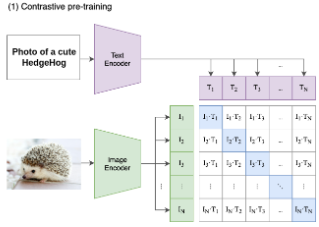
From basic transformers, we can imagine how images are simply just embeddings of pixels that are augmented by their two-dimensional position encoding. CLIP is a contrastive learning framework that unifies image and text by utilizing cross attention, where queries and keys are one of the two modalities. After encoding our data, we’ll feed in multiple images and multiple text embeddings such that we’re matching a text encoding with an image encoding. The contrastive objective is the ability to learn and distinguish proper text and image embeddings. At inference time we can simply feed in one image and list a bunch of possible text outcomes to then determine the outcome.

Other papers discuss special token placeholders such as a [mask] token. Other tokens may be [action] tokens that refer to a command the transformer can make (i.e “Hello there! [shake hand]”). This paper emphasizes the way that transformers operate and a self-constructing graphical neural network where each token input is a node and the strength of connections to other nodes is the weighting done in our query key dot product. While the transformer architecture generally stays the same for each implementation, the tokenization and token embeddings change.

• Tokenization is the process of taking, say language and splitting each word into tokens, or sub-words like "ch" and "sh" into byte pair encodings. Image transformers tokenize through taking small chunks of an image and linearizing them. Often additional tokens are given as registers, or as additional context towards what patch of data is being analyzed in an image.
• Token embeddings are then the way we convert a token into a vector. Pixels or words have to be translated either with existing networks or as in our case, a simple trainable neural network layer. Token embeddings can be infused such as the original token embedding plus a positional embedding. If we want to analyze an image based on a region of interest (ROI) we can use an image embedding + position embedding + ROI embedding. We can also add linguistic embeddings or segment embeddings, truly anything we desire.

Next the paper discusses the differing ways of utilizing fusions in a transformer.

• Early summation was discussed previously in which we conduct an element-wise sum embedding with weights alpha and beta. The position embedding is such an embedding. $$Z=\alpha Z_{a}\bigoplus \beta Z_{b}=MHSA(Q_{ab},K_{ab},V_{ab})$$
• Early Concatenation is simply the concatenation of an input. VideoBERT just fuses text and video feeds with early concatenation to encode a global multimodal context feed. Longer sequences do increase computation complexity. $$Z=Tf(C(Z_{a},Z_{b}))$$
• Hierarchical Attention has us encode with independent transformer streams and then concatenate outputs. $$Z=Tf_{3}(C(Tf_{1}(Z_{a}),Tf_{2}(Z_{b}))$$ Here's what this code may look like:

  self.sa_1 = MultiHeadAttention(n_head_1, head_size_1)
  self.sa_2 = MultiHeadAttention(n_head_2, head_size_2)
  self.sa_3 = MultiHeadAttention(n_head_3, head_size_3)
  x_1 = self.sa_1(self.ln1(x))
  x_2 = self.sa_2(self.ln1(x))
  x = x + self.sa_3(self.ln1(torch.cat(x_1, x_2)))
  

  
• Cross-Attention was already discussed and is simply the query and key being of different modalities. An interesting point about this method is that each modality A is conditioned on the other modality B, however we do not perform cross-modal attention globally and therefore context is lost.
  
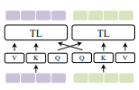
• Cross-Attention to Concatenation fixes this by concatenating two cross attentions and processing a final transformer layer.
  

Task-Agnostic Multimodal Pretraining is essentially the process by which we take unstructured data and feed it into our model and have it predict the next token. This makes our model able to train effectively on unstructured data, learning representations before we transition the model to train on structured, specific tasks.

Knowledge distillation is a fun technique in which we train a smaller model to just act like a larger model by utilizing cross-entropy on the outputs which allows models to be smaller and still similarly powerful. What’s interesting is that we can take a multimodal model and use knowledge distillation to train smaller unimodal models.

Training understanding and discriminative tasks requires an encoder, while generative tasks require both the encoder and decoder. This is true for not just multimodal transformer models but AI in general and is just something I hadn’t thought of lol.

Discovering and adapting latent semantic alignments across modalities is crucial in future tasks.

(2023)A transformer-based representation-learning model with unified processing of multimodal input for clinical diagnostics

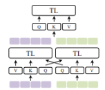
A hierarchical model that utilizes intramodal and intermodal attention learns holistic representations of radiographs and text comprising chief complaints, clinical history and structured clinical laboratory or demographic information. This type of model can help streamline triaging of patients and facilitate the clinical decision-making process.

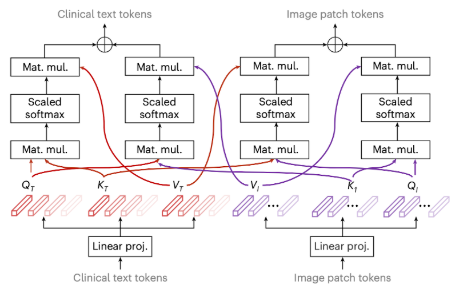
The picture above is a better demonstration of a form of cross-attention used in a hierarchical setting where another attention block can learn from both embeddings. This is considered a “bidirectional multimodal attention layer”, which means that when we train our model, we mask random tokens within and have our model predict based on past and future tokens. This doesn’t help in “predicting”, but for the case of classification we don’t need prediction of the next token, we only need a deep understanding of the data.

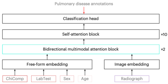
The entire structure involves simple embeddings, two bidirectional multimodal attention blocks stacked, ten self-attention blocks and then a final classification head for the diseases analyzed. Lab data is either tokenized or uses linear projections into an acceptable range (sex may be 0 or 1, age is transformed to be between 0 and 1).

(2023)Continual Self-Supervised Learning: Towards Universal Multi-modal Medical Representation Learning

The idea behind this paper is that we want a “universal” multimodal architecture where the transformer doesn’t care what modality you feed it. This leads to catastrophic forgetting and the authors emphasize the need for continual samples from various modalities to avoid this. There are dimension-specific tokenizers to also help accomplish this goal. This task seems ill-guided, as I don’t know why we’d wish for a universal architecture. Similarly in how our brains work, we have different parts of our brains for different tasks. We can try to get our math compartment to do english, but what’s the point?

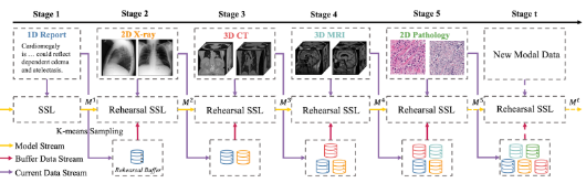
We have to maintain an expensive pipeline and keep feeding in previous samples. This truly stretches the capabilities of transformers in a way that isn’t ideal for the technology, especially given how other multimodal architectures opt for separate backbones per modality.

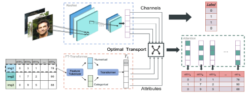
(2023)Tabular Insights, Visual Impacts: Transferring Expertise from Tables to Images

This paper has two modalities, face images and tabular descriptors. They separately encode both modalities before conducting optimal transport. Afterwards a self-attention layer is used before classifying the desired data. This method’s main purpose is to highlight optimal transport theory as a way to better improve mutual information from two modalities. They’re trying to align representations into a shared embedding space.

(2024)Temporal Cross-Attention For Dynamic Embedding And Tokenization Of Multimodal Electronic Health Records

Multimodal clinical time series are incredibly challenging and require dynamic embedding and tokenization schemes to enable transformers to adapt. This paper combines structured, numerical time series data and free-text clinical notes through an adoption of cross-attention to create a joint multimodal temporal representation.

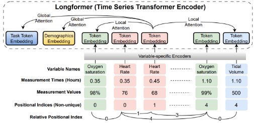
• Flexible positional encoding: Different measurements are taken in different increments (vital signs every minute, labs every 24 hours). Resampling is possible but it may inject bias into data representation. The authors implement non-unique positional indices based on recorded timestamps for each measurement. There is an additional relative positional encoding added to each token embedding used to help capture local token dependencies that help with clusters of measurements and long sequences.
• Learnable time encoding: Time2Vec encodes two model-agnostic vector representations, one being periodic and the other not. The parameters for the periodic and non periodic vectors are learnable.
• Variable-specific encoding: Separate encoders are used for each clinical variable for intra-variable temporal dynamics, and then are concatenated to learn inter-variable correlation and dependencies.

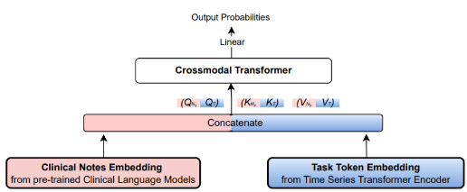
As for the actual model, we’ve seen this method before in our survey being a simple early concatenation that ultimately performed best where Q,K,Vs are calculated for each embedding independently, and then a crossmodal transformer embeds the information into a common latent space for classification.

(2024)Deep Multimodal Learning with Missing Modality: A Survey

Missingness is either handled at a data level or at an architectural level. Here are two methods described in the paper for handling missingness:

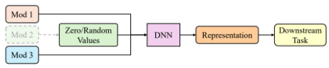
This method just sets any missing modalities to zero.

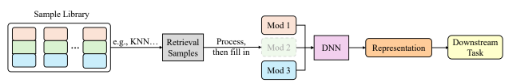
This method samples modalities, and if modalities are missing, it will randomly sample from a similar example via KNN (or some other clustering method) to fill in the missing modality before then randomly removing a sample. This is only really useful for classification and may lead to overfitting. With more missingness, this method degrades in performance.

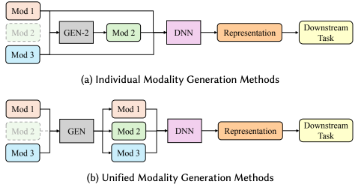
Generative methods are also used for creating modalities for modality imputation. Autoencoders, GANs and Diffusion Models are generally used to construct embeddings. This in my mind is problematic, as best imputation practices are done with simpler tree models, however given the quantity and dimensionality of the data, these ML methods may prove to be better. The paper argues that GANs have been shown to perform better and link to a study, however the study they reference only compare basic implementations of AEs and VAEs to a much more complex implementation of a GAN they call SMIL. Even then the difference in performance was 94% accuracy to 96% accuracy for a MUCH more complicated model.

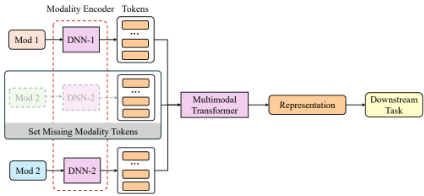
This structure focuses on creating a joint representation through encoding and concatenating modality tokens. This model requires a large amount of data and computing resources to pull off.

Distillation methods seem the most promising on the outset. They try to focus on reconstruction of missing modalities through trying to get a teacher and student model to agree on how to represent missing data in a joint embedding space.

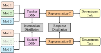
Here we have a teacher helping the student reconstruct a missing modality in the response distillation. However we can also see an intermediate distillation, in which the weights of the models are compared and adjusted to help the student DNN.

From this paper I keep seeing the same idea, basically CLIP where we encode various modalities into the same featurespace, and it makes intuitive sense to me that this approach is best. However this method may create some oversimplifications towards not being able to address small nuances in modality cases. In my field of health, small nuances may be important, and unless there are a substantial number of samples for each small nuance, we have to rely on a model’s ability to generalize tasks for understanding and giving proper diagnosis.

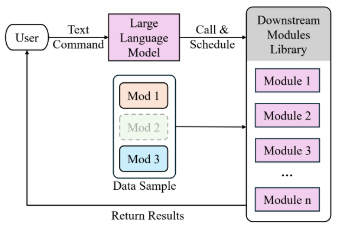
Discrete Scheduler Methods are super interesting in which an LLM takes control over which steps are conducted and analyzed. We can give the LLM abilities to engage with multimodal tools to analyze chest X-rays or separate modality models to come to decisions based on the data. This is the closest and probably most realistic way a robo-doctor could be implemented and trusted. It gives me a lot of ideas!

The issues this paper brings up talk about:

• Hallucinations and artifacts within generated samples.
• If we should generate samples or to simply train models to avoid having to generate at the risk of hallucinating information.
• There is no easy benchmarking for missing modality scenarios, making methods hard to compare to one another.

This was an incredibly in-depth and at time confusing paper on missingness in transformers and I was very happy with the quality of this survey!