My Thesis Work: Multimodal and Synthetic Data

While my thesis is in the cogs of being published, because I still wanted to post about it and talk about it on my blog. This is a cut up version that touches on the major keystones of my work. Originally I was doing a PhD, but decided to master out, so my research is more than a typical master’s thesis in terms of scope.

A big issue in research is utilizing multiple modalities. This is primarily due to lack of supporting data and lack of obvious methods to integrate said data streams together for quality decision-making. I’ll break down this summary into 4 unique sections that tackle multimodal healthcare:

	Synthetic Data	Small Afib Dataset (Tabular)
Multimodal Combinations	Part 1	Part 2
Large MIMIC Dataset (Tabular + Image)	Part 3	Part 4

Part 1: Multimodal Combinations for the Small Afib Dataset

Looking at our first dataset, we have two batches, a first more complete dataset (95% completeness and 24 patients), and a second, drastically less complete dataset (71% completeness and 54). The quality of the data in the second dataset also struggles because it had unexplainably lesser quality correlations. Common strong variables in dataset one were less so in dataset two.

On top of the missingness and already low patient count, we had 102 features to sift through! That means before I could even begin to answer my original question of multimodal combinations, I had to assess what values from each modality were even appropriate to consider.

In small data environments we generally utilize k-fold or leave-one-out cross validation (LOOCV). However this method has a flaw in that it doesn’t allow for a validation split! To fix this we nest our procedure with an additional LOOCV. We have an outer and inner loop now which gives us more flexibility at the cost of slightly less samples, and exponentially more folds to compute.

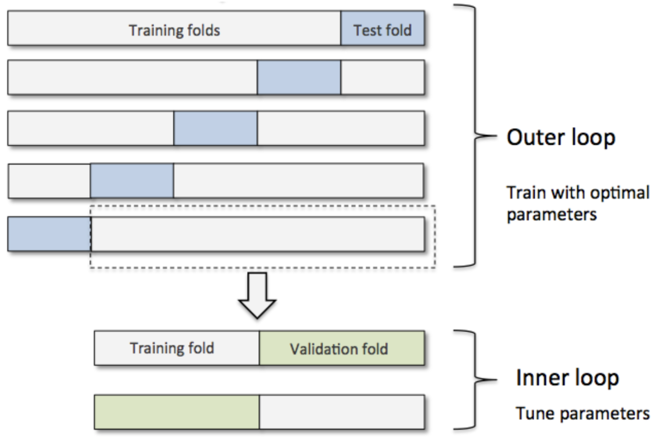
We can add an additional nested loop to add in a “structural” layer by which we conduct feature selection, and the feature set we report as the “best” can then be a combination of best features each iteration consistently ranks as important. SHAP selection is thereby used, as it’s a universal means by which we can assess the strength of variables in a best-fit model.

To focus quickly on the downsides, we ARE dealing with far more computations the more we nest our folds, and the benefits of doing so diminish in most datasets, however in genomics and exploratory research these methods are far more common as the extra rigor in methodology results in stronger and more consistent results in highly volatile datasets. Another factor to consider is that these calculations are parallelizable in so far that every iteration required is irrespective of the calculation prior. Even if we had to conduct 500 different analyses, split over 50 machines, we drastically reduce the complexity of the job.

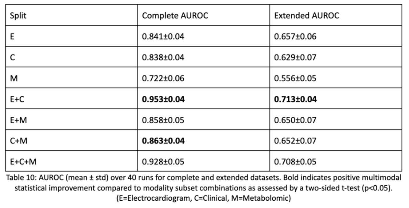
So outside of methodology, what were the results? Of our three modalities we found that the combination of electrocardiogram data and clinical data made the best, statistically significant result. Statistical correctness is done using a two-sided t-test by which we take each LOOCV fold’s AUROC score and compare it to every modality subset’s LOOCV fold AUROC. This shows that multimodal data is beneficial, but not always. The modalities have to be synergistic and non-parallel to contribute. Metabolomic data clearly wasn’t as useful and detracted from model performance. This may have been due to the fact that even though metabolomic data causes downstream effects, having distal upstream causes isn’t as predictive as having causal, bigger impact data.

Part 2: Synthetic Data for the Small Afib Dataset

The next aspect of my research delves into synthetic data generation. Because multimodal data is hard to collect where all data is available, we have to consider that imputing said synthetic data may be the best way to allow for multiple modalities to be incorporated.

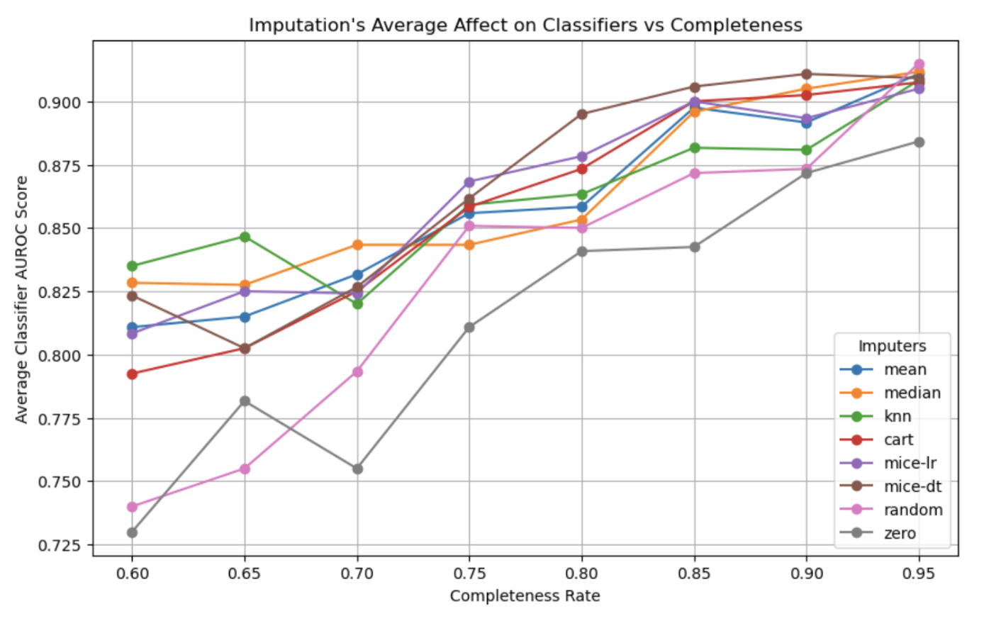
So how do varying imputation methods compare and varying levels of completeness? The answer is complicated. For the most part we find that the type of imputation doesn’t have much effect on the quality of downstream classifications! This is possibly due to the fact that sophisticated non-linear models used in our analysis can encode missingness with poor imputations (zero, mean) and benefit from good imputations (MICE-DT, cart) equally.

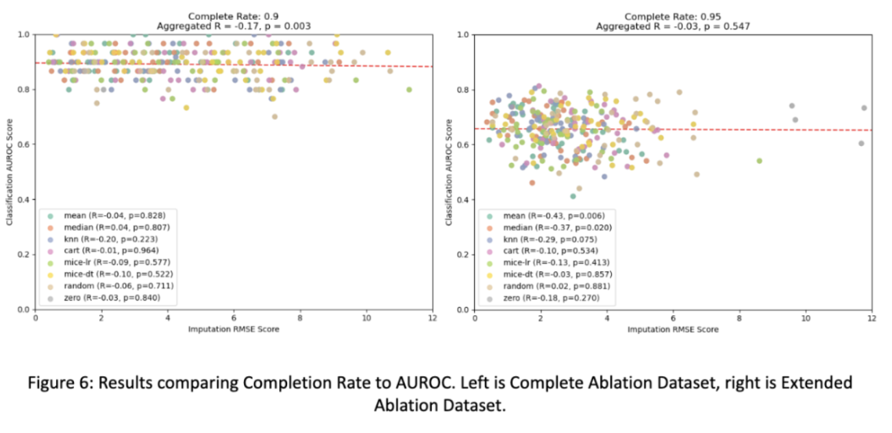
Only as completeness drastically decreases in some cases are methods like zero-only imputation and random imputation actually performing worse than other methods for the small dataset. This finding follows the principal of dropout, where a small amount of missingness can force a model to generalize better than if it had completed data, which may explain this phenomena.

And when taking into account the multimodal aspect of this analysis, we find that modalities unevenly contribute towards accurately imputing the other modality. When electrocardiogram missingness decreases, it is sufficiently imputed by the clinical data, but this relationship doesn’t necessarily hold for the inverse situation. And for the larger (extended) dataset we see that this relationship is reversed in which modality can impute the other.

This is only tested on our Afib dataset, so other multimodal datasets may produce drastically differing results depending on the variable relationships and that is to say, all of these findings need a larger analysis on more multimodal datasets (which are unfortunately hard to come by).

Lastly, we wish to see how well we can impute entirely missing modalities. Here we see that the superior imputer modality for both the small and larger datasets successfully go from a single modality, use past multimodal combinations to IMPROVE single modality predictions to be equal to that of a superior multimodal prediction. This is an incredible finding with many real-world impacts to consider. Before we conduct a surgery, based on clinical values and known future electrocardiogram relationships, we can improve the prediction of a successful surgery! We are doing more with less and this result is incredibly exciting as it opens up avenues for many fields to incorporate this type of study design to improve results across the board!

Part 3: Multimodal Combinations for the MIMIC Dataset

Multimodal data for the mimic dataset is drastically different. We had an image of a radiological PA scan alongside a tabular summation of predictive lab values. While we may have every image in a dataset, corresponding desired lab values are not nearly as common. This drastic reduction in data quality alongside a larger transformer model that requires large sums of data causes a challenge in both experimental design, as well as architectural designs for our large DNN we wish to employ for the problem.

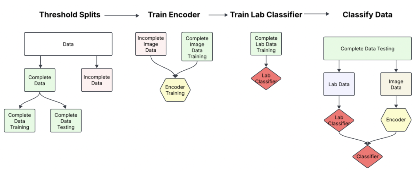
Our solution was this procedure:

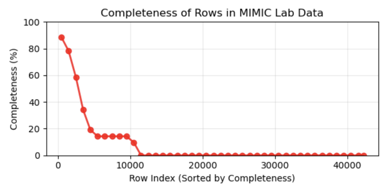
1. Threshold Splits: Find a serviceable threshold by which we may consider the data "complete" and "incomplete". This threshold was devised through determining the missingness threshold by which our lab data had reliable predictive signal. (This threshold was 65% completeness in tabular data)
2. Train Encoder: Using an existing state-of-the-art DINO model, we first finetuned the image encoder on incomplete data. Then we later finetuned the encoder on a subset of completed training data. Because we wish to test how well our model performs GIVEN multimodal data, we split our complete data into training testing and validation sets.
3. Train Lab Classifier: Next we'd, if necessary train a lab classifier to preprocess the complete training lab data. Because the data was already in such a limited form however, this step wasn't practical to train an encoder. For a late fusion model comparison, we'd train a lab classifier at this step to compare performances between our desired joint-fusion model to a baseline late-fusion model.
4. Classify Data: The last step would be to train on our training/validation data and finally test our model's performance.

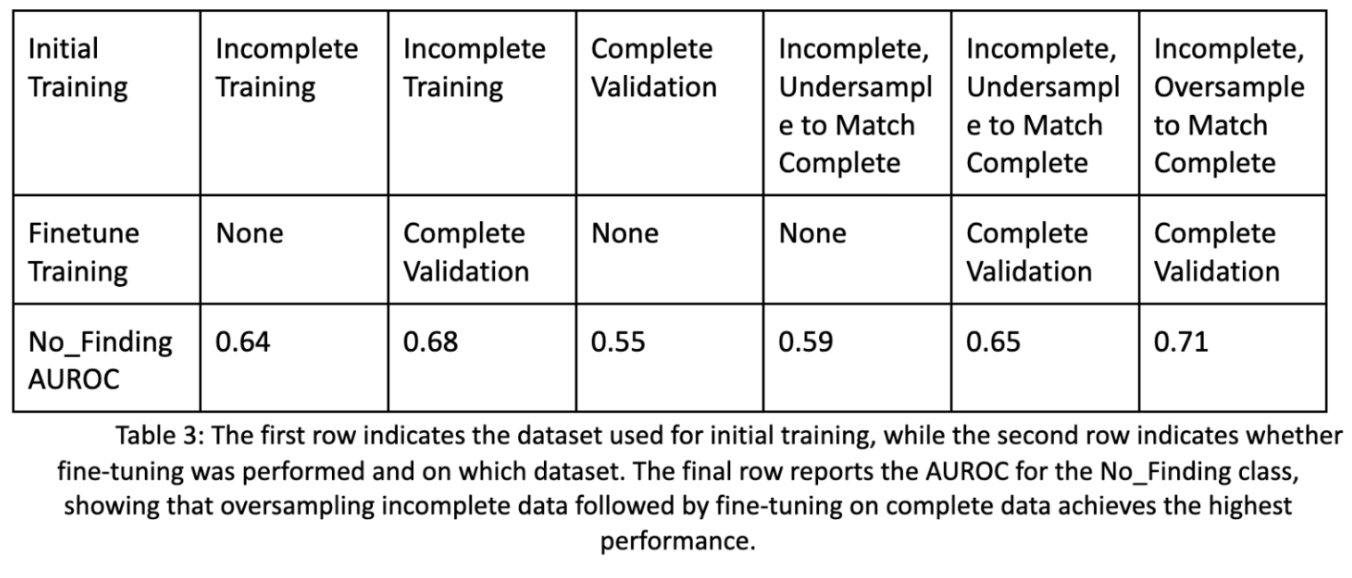
Below are the improvements in performance for a basic image encoder given these additional steps. We see an improvement of 7% from training only on incomplete data, to utilizing our pipeline with additional oversampling. Also note that the complete image data will be sufficiently different in type compared to the incomplete image data, as some diseases with or without certain lab values may be more common.

Below is the architecture utilizing our SOTA DinoV2 encoder and tabular data:

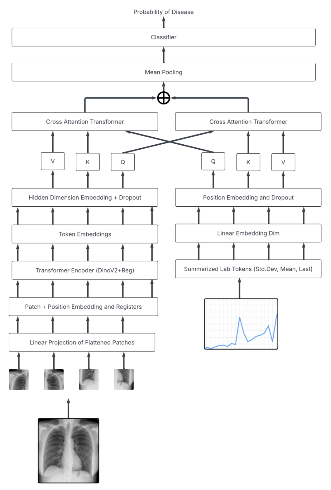
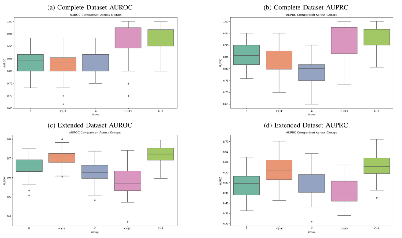
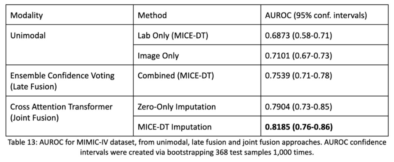
Below are the results by which we see how well unimodal performances are decent, however late fusion performs much better. Then we also find that our joint fusion model with MICE-DT imputation for missing values performs the best. Notice as well, compared to most other DNN papers we have confidence intervals! Firstly, AUROC scores are preferable because they highlight the model’s ability to assign confidence to an estimate and allows practitioners to threshold assessments appropriately. Secondly, we take our batch of 368 test samples and repeatedly sample from them 1,000 times in order to form a statistic about the distribution of the dataset. This bootstrapping method allows us to estimate a spread of accuracy of the model and allows us to determine statistical significance from one model to another.

Part 4: Synthetic Data for the MIMIC Dataset

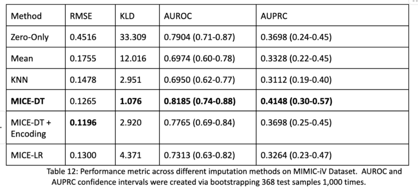
The last elephant in the room is the fact that we used synthetic data in our transformer model! And that the MICE-DT imputation performed better than the Zero-Only imputation model. Isn’t this to be expected? Why were the performances still so close? What about other methods? We actually did impute every model and test their performance as shown below on the same process for the entire dataset. We found that RMSE and KLD were not predictive of downstream AUROC and AUPRC performance metrics. The best models were that of MICE-DT and surprisingly Zero-Only imputation! Zero-Only, as in our tabular data does actually encode meaningful data; missingness.

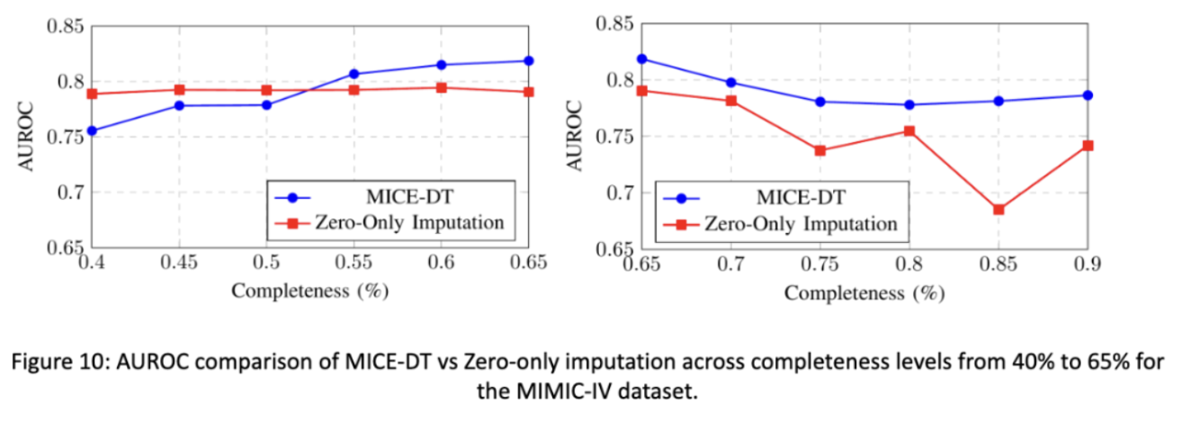
In our final figure shown we see that if we change the completeness of our testing data, the more sparse it is, the better the zero-only imputation transformer outcompetes the mice-dt imputation transformer. In the opposite direction we see that MICE-DT performs better when data is closer to being filled in. This makes intuitive sense, and tells researchers to consider future directions of data support in how they impute data. If you plan on having less data in the future, zero-only imputation may be better and visa versa.

Conclusion

Research is a lot of fun! It’s so enjoyable to work on hard problems and to work with talented inquisitive people on subjects that really matter! The thesis was a blast and I’m glad I got that experience, as no classroom could emulate an academic research environment. Every week I’d present results, get questioned on said results and decide how to move forward. Honestly the hardest part was just succinctly writing everything I learned and communicating that, but if a scientist cannot communicate results, then what was the point of having done said research in the first place?

This blog helps serve that purpose, and thank you so much for reading and hopefully having an enjoyable time, maybe you learned something? If not, you’re a wizard because so much of my research had unexpected results that really interested me to continue studying and researching in the future!

See you next time :)

P.S: I know there are weaknesses that in foresight I wish I knew about. I could’ve utilized permutation testing for my small sample size data to test performance differences without bias, and I wish I had more generalizable datasets to work off of. I will do this in the future!